During my time on the red team, we continually discussed the role of matched filters in everything from GPS to fire control radars. While I’m having a blast at DARPA where I work in cyber, I wanted to review an old topic and put MATLAB’s phased array toolbox to the test. (Yes, radar friends this is basic stuff. I’m mostly writing this to refresh my memory and remember how to code. Maybe a fellow-manager might find this review helpful, but if you are in this field, there won’t be anything interesting or new below.)
Why use matched filters?
Few things are more fundamental to RADAR performance than the fact that probability of detection increases with increasing signal to noise ratio (SNR). For a deterministic signal in white Gaussian noise (a good assumption as any regarding background noise but the noise does not need to be Gaussian for a matched filter to work), the SNR can be maximized at the receiver by using a filter matched to the signal.
One thing that always confused me about matched filters was that they really aren’t a type of filter, but more of a framework that aims to reduce the effect of noise which results in a higher signal to noise ratio. One way I’ve heard this described is that the matched filter is a time-reversed and conjugated version of the signal.
The math helps to understand what is going on here. In particular, I want to derive that the peak instantaneous signal power divided by the average noise power at the output of a matched filter is equal to twice the input signal energy divided by the input noise power, regardless of the waveform used by the radar.
Suppose we have some signal $r(t) = s(t) + n(t)$ where $n(t)$ is the noise and $s(t)$ is the signal. The signal is finite, with duration $T$ and let’s assume the noise is white gaussian noise with spectral height $N_0/2$. If the aggregated signal is input into a filter with impulse response $h(t)$ and the resultant output is $y(t)$ you can write the signal and noise outputs ($y_s$ and $y_n$) in the time domain:
$$ y_s(t) = \int_0^t s(u) h(t-u)\,du $$
$$ y_n(t) = \int_0^t n(u) h(t-u)\,du $$
Since we want to minimize the SNR, we expand the above:
$$\text{SNR} = \frac{y_s^2(t)}{E\left[y_n^2(t) \right]}$$
$$ = \frac{ \left[ \int_0^t s(u) h(t-u)\,du \right]^2}{\text{E}\left[ \int_0^t n(u) h(t-u)\,du \right]^2}$$
The denominator can be expanded:
$$\text{E} \left[y_n^2(t) \right] = \left[ \int_0^t n(u) h(t-u)\,du \int_0^t n(v) h(t-v)\,dv \right] $$
Or
$$ \int_0^t \int_0^t E [ n(u) n(v) ] h(t-u) h(t-v) du\,dv $$
We can further simplify this by invoking a standard white noise model:
$$ E[y_n^2] = \frac{N_0}{2} \int_0^t \int_0^t \delta(u-v) h(t-u) h(t – v) du\,dv $$
Which simplifies nicely to:
$$ \frac{N_0}{2} \int_0^t h^2 (t – u) du $$
Now all together we get:
$$ SNR = \frac{ \left[ \int_0^t s(u) h(t-u)\,du \right]^2 }{\frac{N_0}{2} \int_0^t h^2 (t – u) du } $$
In order to further simplify, we employ the Cauchy-Schwarz Inequality which says, for any two points (say $A$ and $B$) in a Hilbert space,
$$ \langle A, B \rangle^2 \leq |A|^2 |B|^2 \text{,}$$
and is only equal when $A = k\,B$ where $k$ is a constant. Applying this, we can then look at the numerator:
$$ \left| \int_0^t s(u)\,q(u) du \right|^2 \leq \int_0^t s^2(u) du \int_0^t q^2(u) du $$
and equality is acheived when $k\,s(u) = q(u)$.
If we pick $h(t-u)$ to be equal to $k\,s(u)$, we can write our optimal SNR as:
$$ SNR^{\text{opt}} (t) = \frac{k \left[ \, \int_0^t s^2 (u) duN \right]^2 }
{
\frac{N_0 k^2}{2}
\int_0^t s^2(u) du
} = \frac{\int_0^t s^2(u) du
}{
N_0/2
}$$
Since $s(t)$ always has a finite duration $T$, then SNR is maximized by setting $t=T$ which provides the well known formula:
$$SNR^{\text{opt}} = \frac{\int_0^T s^2(u) du}{N_0/2} = \frac{2 \epsilon}{N_0}$$
So, what can we do with matched filters?
Let’s look at an example that compares the results of matched filtering with and without spectrum weighting. (Spectrum weighting is often used with linear FM waveforms to reduce sidelobes.)
The most simple pulse compression technique I know is simply shifting the frequency linearly throughout the pulse. For those not familiar with pulse compression, a little review might be helpful. One fundamental issue in designing a good radar system is it’s capability to resolve small targets at long ranges with scant separation. This requires high energy, and the easiest way to do that is to transmit a longer pulse with enough energy to detect a small target at long range. However, a long pulse degrades range resolution. We can have our cake and eat it to if we encode a frequency change in the longer pulse. Hence, frequency or phase modulation of the signal is used to achieve a high range resolution when a long pulse is required.
The capabilities of short-pulse and high range resolution radar are significant. For example, high range resolution allows resolving more than one target with good accuracy in range without using angle information. Many other applications of short-pulse and high range resolution radar are clutter reduction, glint reduction, multipath resolution, target classification, and Doppler
tolerance.
The LFM pulse in particular has the advantage of greater bandwidth while keeping the pulse duration short and envelope constant. A constant envelope LFM pulse has an ambiguity function similar to that of the square pulse, except that it is skewed in the delay-Doppler plane. Slight Doppler mismatches for the LFM pulse do not change the general shape of the pulse and reduce the amplitude very little, but they do appear to shift the pulse in time.
Before going forward, I wanted to establish the math of an LFM pulse. With a center frequency of $f_0$ and chirp slope $b$, we have a simple expression for the intra-pulse frequency shift:
$$
\phi (t) = f_0 \, t + b\,t^2
$$
If you take the derivative of the phase function, instantaneous frequency is:
$$ \omega_i (t) = f_0 + 2\,b\,t. $$
For a chirp pulse width in the interval $[0, T_p]$, $\omega_i(0) = f_0$ is the minimum frequency and $\omega_i(T_P) = f_0 + 2b\,T_P$ is the maximum frequency. The sweep bandwidth is then $2\,bT_p$ and if the unit pulse is $u(t)$ a single pulse could be described as:
$$ S(t) = u(t) e^{j 2 \pi (f_0 t + b t^2)} \text{.}$$
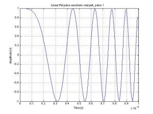
I learn by doing, so I created a linear FM waveform with a duration of 0.1 milliseconds, a sweep bandwidth of 100 kHz, and a pulse repetition frequency of 5 kHz. Then, we will add noise to the linear FM pulse and filter the noisy signal using a matched filter. We will then observe how the matched filter works with and without spectrum weighting.
Which produces the following chirped pulse,
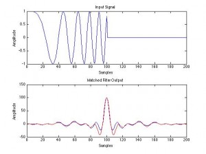
From here, we create two matched filters: one with no spectrum weighting and one with a taylor window. We can see then see the signal input and the matched filter output:
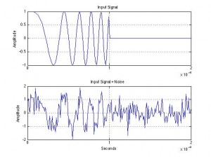
To really see how this works we need to add some noise:
{aaa01f1184b23bc5204459599a780c2efd1a71f819cd2b338cab4b7a2f8e97d4} Create the signal and add noise.
sig = step(hwav);
rng(17)
x = sig+0.5*(randn(length(sig),1)+1j*randn(length(sig),1));
And we can see the impact noise has on the original signal:
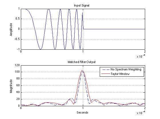
and the final output (both with and without a Taylor window):
The Ambiguity Function
While it is cool to see the matched filter working, my background is more in stochastic modeling and my interest is in the radar ambiguity function — which is a much more comprehensive way to examine the performance of a matched filter. The ambiguity function is a two-dimensional function of time delay and Doppler frequency $\chi(\tau,f)$ showing the distortion of a returned pulse due to the receiver matched filter due to the Doppler shift of the return from a moving target. It is the time response of a filter matched to a given finite energy signal when the signal is received with a delay $\tau$ and a Doppler shift $\nu$ relative to the nominal values expected by the filter, or:
$$
|\chi ( \tau, \nu)| = \left| \int_{-\infty}^{\infty} u(t)u^* (t + \tau) exp(j 2 \pi \nu t) dt \right| \text{.}
$$
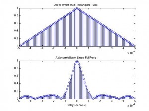
What is the ambiguity function of an uncompressed pulse?
For an uncompressed, rectangular, pulse the ambiguity function is relatively simple and symmetric.
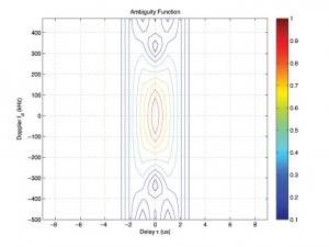
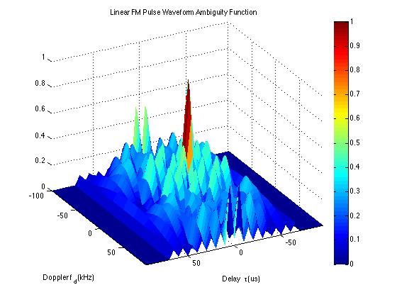
What does the ambiguity function look like for the LFM pulse described above?
If we compare two pulses, each with a dutycycle of one (PRF is 20 kHz, and pulsewidth is 50 µs), we can see their differing ambiguity functions:
If we look at the ambiguity function of an LFM pulse with the following properties:
SampleRate: 200000
        PulseWidth: 5e-05
               PRF: 10000
    SweepBandwidth: 100000
    SweepDirection: 'Up'
     SweepInterval: 'Positive'
          Envelope: 'Rectangular'
      OutputFormat: 'Pulses'
         NumPulses: 5
then we can see how complex the surface is:
.
References
- http://www.ece.gatech.edu/research/labs/sarl/tutorials/ECE4606/14-MatchedFilter.pdf
- Matlab help files
Leave a Reply