My twelve year old daughter is working a science fair project on electricity and home usage. As part of her project, we have been taking lots of measurements of the electricity usage throughout our house. This provided a great opportunity to talk about smoothing and for me to publicly work through my resultant confusion. Smoothing is necessary because noise is so ubiquitous. Even if you could remove all the noise from an input device, you’ll still have a certain degree of uncertainty because the world is not fundamentally deterministic.1 Even more, smoothing is such a general problem that it traverses nearly all aspects of signal processing.
Filters are the general tool that allow engineers to work with uncertainty.2 In general, a filter is device or process that removes unwanted components or features from a signal. I like to think of a filter as a tool that takes a series of observations, and attempts to find the most likely signal that generated them. They are then a necessary tool in a noisy world. All sensors require filters, and filters play an essential (yet somehow hidden) role in our lives. [Alan Zucconi] had a great blog post on this that I leverage for the content below.
The ability to recover a signal that has been corrupted by noise depends on the type of noise and the relative proportion of noise and signal (often called the SNR or signal to noise ratio). One of the most common problems is to remove additive noise, uniformly distributed also often called Gaussian white noise. Here the noise is totally independent from the original signal. Additive uniform noise is often the result of an external interference.
There are many types of filters defined by what assumptions they make about the signal. Most all filters deal in the frequency domain, while some filters in the field of image processing do not. Some examples of filters include linear or non-linear, time-invariant or time-variant, causal or not-causal3, analog or digital, discrete-time (sampled) or continuous-time. Linear filters fall several broad categories based on what frequencies are allowed to pass. The filter passes the passband and rejects the stopband. Filters are divided into these categories and you will hear these terms used frequently in the electrical engineering community:
Low-pass filter – low frequencies are passed, high frequencies are attenuated.
High-pass filter – high frequencies are passed, low frequencies are attenuated.
Band-pass filter – only frequencies in a frequency band are passed.
Band-stop filter or band-reject filter – only frequencies in a frequency band are attenuated.
Notch filter – rejects just one specific frequency – an extreme band-stop filter.
Comb filter – has multiple regularly spaced narrow passbands giving the bandform the appearance of a comb.
All-pass filter – all frequencies are passed, but the phase of the output is modified.
The following picture helps make sense of these terms:

Moving Average
One of the most simple filters is the ability attenuate additive noise is called the moving average filter. A Moving average is based on the assumption that independent noise is not going to change the underlying structure of the signal, so averaging a few points should attenuate the contribution of the noise. The moving average calculates the average of its neighboring points for each point in a signal. For example, from three points the filtered signal is given by averaging:
$$F_i = \frac{N_{i-1}+N_{i}+N_{i+1}}{3}$$
If all the observations are available, we can define moving average with window size $N=2k+1$ as:
$$F_i = \frac{1}{N} \sum_{j = -k}^{+k} S_{i-j}$$
While the moving average technique works well for continuous signals, it is likely to alter the original signal more than the noise itself if there are large discontinuities. Moving average is the optimal solution with linear signals which are affected by additive uniform noise.
Centered Moving Average
A moving average introduces a constraint over $N$: it has to be an odd number. This is because a moving average requires an equal number of points $k$ before and after the center point: $N_i$. Since we count $N_i$ itself, we have $2k+1$ points, which is always odd. If we want to use moving average with an even number of points ($M = 2k$), we have two possibilities. For example, if $k=2$ and $MA$ is the moving average:
$$
MA^L_4=\frac{N_{i-2} + N_{i-1} + N_{i}+ N_{i+1} }{4}
$$
$$
MA^R_4=\frac{N_{i-1} + N_{i} + N_{i+1}+ N_{i+2} }{4}
$$
Both these expressions are valid, and there is no reason to prefer one over the other. For this reason, we can average the together to get a centered moving average. This is often referred as $2\times 4 MA$.
$$
2\times 4 MA=\frac{1}{2} \left[ \frac{1}{4}\left(N_{i-2} + N_{i-1} + N_{i} + N_{i+1} \right)+ \frac{1}{4}\left( N_{i-1} + N_{i} + N_{i+1} + N_{i+2} \right) \right]=
$$
$$
=\frac{N_{i-2}}{8} + \frac{N_{i-1}}{4} + \frac{N_{i}}{4}+\frac{N_{i+1}}{4}+\frac{N_{i+2}}{8}
$$
This is very similar to a moving average centered on $N_i$, but it helps pave the way for the next concept.
Weighted Moving Average
Moving average treats each point in the window with the same importance. A weighted moving average values points further away from the signal, $S_i$, less by introducing a weight $W_j$ for each time step in the window:
$$F_i = \sum_{j = -k}^{+k} S_{i-j} W_{k+j}$$
with the additional constraint that all $W_j$ must sum up to $1$. Looking back at the repeated average, we can now say that $2\times 4 MA$ is equal to a weighted moving average with weights $\frac{1}{8},\frac{1}{4},\frac{1}{4},\frac{1}{2}$.
The weighted moving average is more powerful, but at the cost of more complexity. It is actually just the beginning of more complex smoothing operations, such as the convolution operator.4
Convolution
At its most basic, convolution is a weighted average with one function constituting the weights and another the function to be averaged. I’ve used convolutions in aerodynamics, digital signal processing and applied probability. It comes up everywhere. Technically, it takes two functions and produces the integral of the pointwise multiplication of the two functions as a function of the amount that one of the original functions is translated. While convolutions are a very powerful operation, we are interested in the ability for convolutions to be a “weighted sum of echoes” or “weighted sum of memories”. They accomplish this by smearing/smoothing one signal by another or they reverse, shift, multiply and sum two inputs. To understand this better, consider two inputs:
DATA: quantities certainly corrupted by some noise – and at random positions (e.g. time or space)
PATTERN: some knowledge of how information should look like
From these, the convolution of DATA with (the mirror symmetric of the) PATTERN is another quantity that evaluates how likely it is that it is at each of the positions within the DATA.
Convolution provides a way of `multiplying together’ two arrays of numbers, generally of different sizes, but of the same dimensionality, to produce a third array of numbers of the same dimensionality. In this sense, convolution is similar to cross-correlation, and measures the log-likelihood under some general assumptions (independent Gaussian noise). In general, most noise sources are very random and approximated by a normally distribution, so the PATTERN often used is the Gaussian kernel.
There are some great explanations of the intuitive meaning of convolutions on quora and stack overflow. I loved this interactive visualization. There is a great example using convolution with python code at matthew-brett.github.io.
For me, it always helps to work a real example. If a 2-D, an isotropic (i.e. circularly symmetric) Gaussian has the form:
$$
G(x,y)={\frac {1}{\sigma^2 {2\pi}}}e^{-\frac{x^2+y^2}{2\,\sigma^2}}
$$
For Gaussian smoothing, we use this 2-D distribution as a ‘point-spread’ function and convolution. This is often done to smooth images. Since the image is stored as a collection of discrete pixels we need to produce a discrete approximation to the Gaussian function before we can perform the convolution. In theory, the Gaussian distribution is non-zero everywhere, which would require an infinitely large convolution kernel, but in practice it is effectively zero more than about three standard deviations from the mean, so we can work with some reasonably sized kernels without losing much information. In order to perform the discrete convolution, we build a discrete approximation with $\sigma=1.0$.
$$
\frac{1}{273}\,
\begin{bmatrix}
1 & 4 & 7 & 4 & 1 \\
4 & 16 & 26 & 16 & 4 \\
7 & 26 & 41 & 26 & 7 \\
4 & 16 & 26 & 16 & 4 \\
1 & 4 & 7 & 4 & 1 \\
\end{bmatrix}
$$
The Gaussian smoothing can be performed using standard convolution methods. The convolution can in fact be performed fairly quickly since the equation for the 2-D isotropic Gaussian shown above is separable into x and y components. Thus the 2-D convolution can be performed by first convolving with a 1-D Gaussian in the $x$ direction, and then convolving with another 1-D Gaussian in the $y$ direction.5
The effect of Gaussian smoothing on an image is to blur an image similar to a mean filter. The higher the standard deviation of the Gaussian, the more blurry a picture will look. The Gaussian outputs a weighted average of each pixel’s neighborhood, with the average weighted more towards the value of the central pixels. This is in contrast to the mean filter’s uniformly weighted average and what provides more subtle smoothing and edge-preservation by convolution when compared with a mean filter. Here is the result of a 5px gaussian filter on my picture:

One of the principle justifications for using the Gaussian as a smoothing filter is due to its frequency response. In this sense, most convolution-based smoothing filters act as lowpass frequency filters. This means that their effect is to remove high spatial frequency components from an image. The frequency response of a convolution filter, i.e. its effect on different spatial frequencies, can be seen by taking the Fourier transform of the filter. Which brings us to . . .
The Fast Fourier Transform
The Fourier transform brings a signal into the frequency domain where it is possible to reduce the high frequency components of a signal. Because it operates in the frequency domain, Fourier analysis smoothes data using a sum of weighted sine and cosine terms of increasing frequency. The data must be equispaced and discrete smoothed data points are returned. While considered a very good smoothing procedure, fourier analysis only works when the number of points is a power of 2 or you’ve padded the data with zeros. Other advantages are the ability for a user to choose cutoff and it can be efficient since only the coefficients needed to be stored store the coefficients rather than the data points. Essentially, you rebuild the signal by creating a new one by adding trigonometric functions.
When the Fourier transform is computed practically, the Fast Fourier Transform (FFT) is used. First, no one wants an approximation built by infinite sums of frequencies, so we use a discrete Fourier transform (DFT). The FFT works by factorizing the DFT matrix into a product of sparse (mostly zero) factors. Due to the huge applications of FFTs, this has been a very active area of research. Importantly, modern techniques to compute the FFT operate at $O(n \log{n})$, compared with the naïve transform of N points in the naive way that would take $O(N^2)$ arithmetical operations.
In practice an analyst will take a FFT followed by reduction of amplitudes of high frequencies, followed by IFFT (inverse FFT).
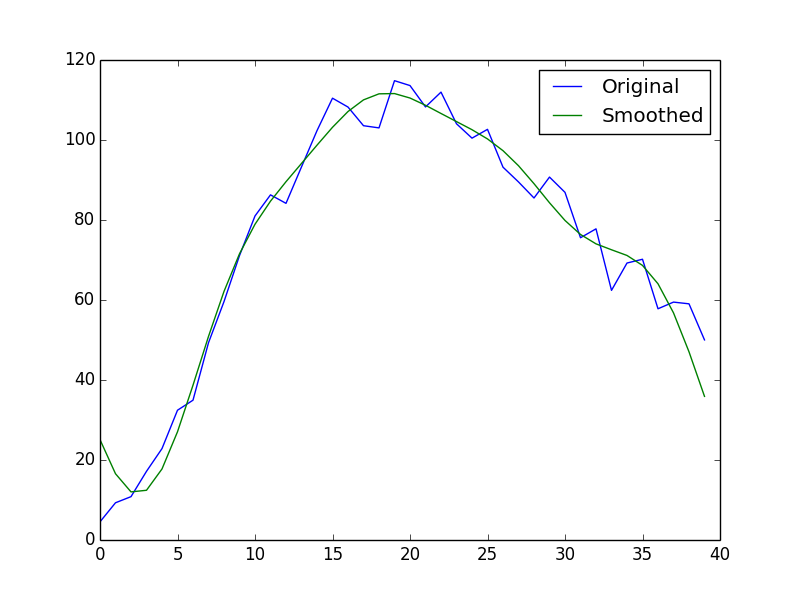
A little bit of python (helped by numpy) can show how this in action:
x = np.arange(40)
y = np.log(x + 1) * np.exp(-x/8.) * x**2 + np.random.random(40) * 15
rft = np.fft.rfft(y)
rft[5:] = 0   # Note, rft.shape = 21
y_smooth = np.fft.irfft(rft)

plt.plot(x, y, label='Original')
plt.plot(x, y_smooth, label='Smoothed')
plt.legend(loc=0).draggable()
plt.show()
Savitzky-Golay filter
Remember the Chuck Wagon burger in school that incorporated a little bit of every food from the week before in it?
The Savitzky–Golay filter uses nearly everything we have talked about above. It first convolves data by fitting successive sub-sets of adjacent data points with a low-degree polynomial by the method of linear least squares.
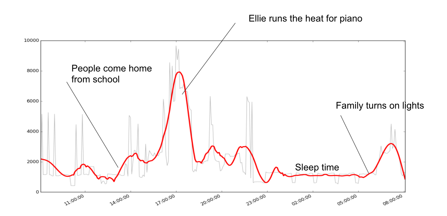
Because python gives you a set of tools that work out of the box, I went ahead and used this one to give to my daughter for her science fair. You can see my code below, but it generated this plot showing electricity usage in our house over 10 days smoothed by Savitzky-Golay windows length 51, and 6th order polynomial.
Kálmán filter
Ok, if you have survived this far, I’ve saved the best for last. I’ve used Kalman filters more than any other tool and they really combine everything. Just this last July, R. E. Kálmán passed away. At the heart of the Kalman filter is an algorithm that uses a series of measurements observed over time, containing statistical noise and other inaccuracies to produces estimates of unknown variables. The Kalman filter ‘learns’ by using Bayesian inference and estimating a joint probability distribution over the variables for each timeframe.
My background with the Kalman filter comes from its applications in guidance, navigation, and control of vehicles, particularly aircraft and spacecraft. The most famous early use of the Kalman filter was in the Apollo navigation computer that took Neil Armstrong to the moon and back.
The Kalman filter permits exact inference in a linear dynamical system, which is a Bayesian model similar to a hidden Markov model where the state space of the latent variables is continuous and where all latent and observed variables have a Gaussian distribution.
Computing estimates with the Kalman filter is a two-step process: a prediction and update. In the prediction step, the Kalman filter produces estimates of current state variables and their uncertainties. Once the outcome of the next measurement (necessarily corrupted with some amount of error, including random noise) is observed, these estimates are updated using a weighted average, with more weight being given to estimates with higher certainty. The algorithm is recursive and can run in real time, using only input measurements and the previously calculated state and its uncertainty matrix; no additional past information is required.
I would write more about it here, but this article by Ramsey Faragher is better than anything I could produce to give an intuitive view of the Kalman filter. This article “How a Kalman filter works in Pictures” is also incredible.
According to Greg Czerniak Kalman filters can help when four conditions are true:
1. You can get measurements of a situation at a constant rate.
2. The measurements have error that follows a bell curve.
3. You know the mathematics behind the situation.
4. You want an estimate of what’s really happening.
He provides an example showing the ability for a Kalman filter to remove noise from a voltage signal:
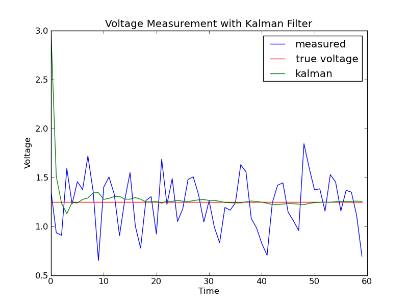
You can find his code here.
Usage
In general, if you want to use a serious filter, I like the Savitzky-Golay and Kalman filter. The Savitzky-Golay is best for smoothing data. The idea behind the Savitzky-Golay smoothing filter is to find a filter that preserves higher-order moments while smoothing the data. It reduces noise while maintaining the shape and height of peaks. Unless you have special circumstances that you want to overcome, use Savitzky-Golay. Of course the Kalman filter could do this. However it is a tool with massive scope. You can pull signals out of impossible noisescapes with Kalman, but it takes a lot of expertise to grasp when it’s appropriate, and how best to implement it.
In some cases, the moving average, or weighted moving average, is just fine, but it bulldozes over the finer structure.
References
I’m so not an expert on filters. If anything above is (1) wrong or (2) needs more detail, see these references:
- E. Davies Machine Vision: Theory, Algorithms and Practicalities, Academic Press, 1990, pp 42 – 44.
- R. Gonzalez and R. Woods Digital Image Processing, Addison-Wesley Publishing Company, 1992, p 191.
- R. Haralick and L. Shapiro Computer and Robot Vision, Addison-Wesley Publishing Company, 1992, Vol. 1, Chap. 7.
- B. Horn Robot Vision, MIT Press, 1986, Chap. 8.
- D. Vernon Machine Vision, Prentice-Hall, 1991, pp 59 – 61, 214.
- Whittaker, E.T; Robinson, G (1924). The Calculus Of Observations. Blackie & Son. pp. 291–6. OCLC 1187948.. “Graduation Formulae obtained by fitting a Polynomial.”
- Guest, P.G. (2012) [1961]. “Ch. 7: Estimation of Polynomial Coefficients”. Numerical Methods of Curve Fitting. Cambridge University Press. pp. 147–. ISBN 978-1-107-64695-7.
- Savitzky, A.; Golay, M.J.E. (1964). “Smoothing and Differentiation of Data by Simplified Least Squares Procedures”. Analytical Chemistry. 36 (8): 1627–39.
- Savitzky, Abraham (1989). “A Historic Collaboration”. Analytical Chemistry. 61 (15): 921A–3A.
Code
I generally write these posts to share my code:
Footnotes
- For friends who have studied physics: Schrödinger’s equation induces a unitary time evolution, and it is deterministic, but indeterminism in Quantum Mechanics is given by another “evolution” that the wavefunction may experience: wavefunction collapse. This is the source of indeterminism in Quantum Mechanics, and is a mechanism that is still not well understood at a fundamental level. For a real treatment of this, check out Decoherence and the Appearance of a Classical World in Quantum Theory. ↩
- Math presents a very different understanding of filters when compared to signal processing where a filter is in general a special subset of a partially ordered set. They appear in order and lattice theory, but can also be found in topology whence they originate. The dual notion of a filter is an ideal. ↩
- A filter is non-causal if its present output depends on future input. Filters processing time-domain signals in real time must be causal, but not filters acting on spatial domain signals or deferred-time processing of time-domain signals. ↩
- See Functional Analysis for more details on how to show equivalence. ↩
- The Gaussian is in fact the only completely circularly symmetric operator which can be decomposed like this. ↩
Leave a Reply