Shapeoko Troubles
I recently encountered an issue when generating a grid of holes for workbench. I had recently planed down an old workbench from our house in New Jersey. I was planning on 20 mm holes spaced in a grid with 96mm spacing to match the festool MFT table. I’m hoping to use the available array of cool attachments and eventually add the aluminum profile to the side. For example, an MFT table can be used as a bench with a variety of different attachments, such as clamping elements and stops.
Unfortunately, the holes didn’t create a proper grid and the spacing was off. I used a CNC machine to cut the holes, but I noticed that they were off. Just looking at it showed that each row had fairly consistent spacing, but the start of the rows varied in the X direction.
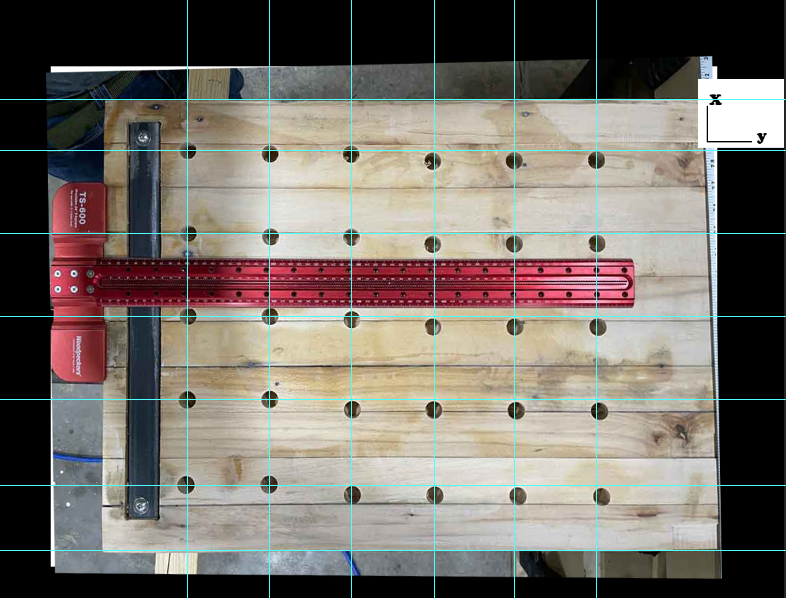
To accomplish a 96 mm grid, the g-code was programmed to start at the bottom of the workpiece and move across in a row. This process was then supposed to be repeated until the entire grid was cut. However, as I mentioned earlier, I encountered some issues with the spacing of the holes and had to troubleshoot the problem.
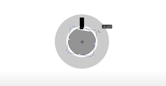
One theory I became aware of online (thanks gdon_2003, Julien, LiamN, SLCJedi and WillAdams) is that set screws are a part of Shapeoko drive system and a loose set screw can cause this type of behavior. That’s because the set screws transfer motion from the motor shafts to the pulleys, which rotate against the belts. They are intended to be pushed tightly against the flat spot on the motor shaft, causing the pulley to turn with the motor. If the set screw becomes loose, the pulley may turn independently of the motor before snapping into place, which can cause issues with the motion of the machine. This may show up as flat spots on circles or other imperfections in projects. You can see why a loose set screw is bad as captured in the screenshot below from this youtube video by See-N-C.
Doing some Math
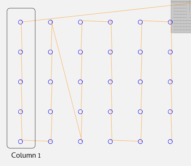
In order to do some analysis on what happened, I needed to register the image and get the location of the points.
The drawpoint command in MATLAB is a function that allows you to draw a single point on an image or plot. You can specify the coordinates of the point on an image using the mouse to record position. Using drawpoint, I recorded the coordinates of the center point of each circle and put this information in a struct. I then wrote code to turn the struct into two arrays: one for the x coordinates and one for the y coordinates. This allowed me to easily analyze the variance in the x coordinates for each column and the variance in the y coordinates for each row.
I was also able to use the drawpoint command in MATLAB to mark points on the ruler captured in the image. This allowed me to easily record the coordinates of the points and then do the math and convert the distances between the points from pixels to millimeters.
I used the pdist2 function in Matlab to calculate the Euclidean distances between my two sampled points and then converted the distances to the desired units through a conversion factor of 610 mm/523.4087 px.
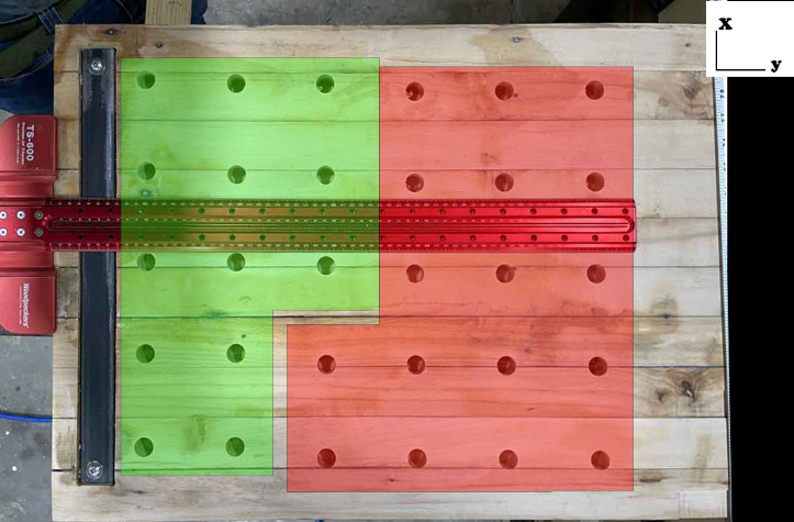
Since the job started at the upper right and progressed down and across, we could look at the variance throughout the job. The variance in the x direction seemed to increase in the last four columns:
| x | 1.261 | 0.3603 | 0.5854 | 0.7656 | 3.2425 | 3.963 |
|---|
The variance in the y direction was much bigger across the rows and also increased as the job progressed. I used this MATLAB to generate this: makemm(var(y(:,:),0,2))
| y | 24.7537 | 24.5736 | 30.6232 | 35.2467 | 36.3425 |
|---|
To generate the ideal points based on a 96 mm grid, I wrote a function that takes in two inputs, iX and iY, which represent the starting x and y coordinates, respectively. The function first initializes two matrices, X and Y, to store the calculated x and y coordinates for each point. Then, it defines a conversion factor, cf, which is used to convert the units from millimeters to pixels.
Next, the function uses a nested for loop to iterate through each column and row of the matrices. For each iteration, the function calculates the x and y coordinates of the current point by adding the starting coordinates (iX and iY) to the appropriate offsets, which are determined by the loop variables and the conversion factor. The calculated x and y coordinates are then stored in the corresponding elements of the X and Y matrices.
To calculate the root mean squared (RMS) error, I subtracted the actual coordinates from the ideal coordinates to find the error in both the x and y directions and then took the square root of the mean of the squared errors in both directions.
| 1 | 2 | 3 | 4 | 5 | 6 | |
|---|---|---|---|---|---|---|
| 1 | 0 | 3.6413 | 4.8678 | 12.5796 | 12.8476 | 12.0532 |
| 2 | 1.2986 | 4.7147 | 4.9236 | 13.6365 | 13.8841 | 12.3934 |
| 3 | 1.604 | 1.4784 | 5.262 | 13.2722 | 13.5265 | 13.8716 |
| 4 | 2.6114 | 2.5362 | 14.1002 | 14.2195 | 14.8988 | 16.2787 |
| 5 | 6.1564 | 6.0407 | 17.3673 | 17.3558 | 18.8129 | 19.6045 |
You can see the error increasing as the job progresses, but the major error starts in column 4-6, supported by a big jump in column 3, row 4, which supports the idea that the screw isn’t seating well resulting in slippage.
Overall, doing this math allowed me to see what was really going on. By adjusting for the variance at 4,3:
Be the first to write a comment.