“Room Temperature” Superconductor?
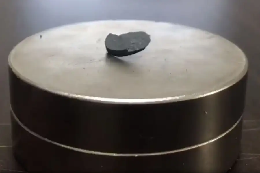
Note: these results are still new and will need to be replicated and further studied by the scientific community. This whole thing may be nonsense, but I did some thinking on the impact if it’s true. Researchers from Korea University have synthesized a superconductor that works at ambient pressure and mild oven-like temperatures (like 260 … Read more