Quick(ish) Price Check on a Car

So, is it a good price?

With my oldest daughter heading off to college soon, we’ve realized that our family car doesn’t need to be as large as it used to be. We’ve had a great relationship with our local CarMax over the years, and we appreciate their no-haggle pricing model. My wife had her eyes set on a particular model: a 2019 Volvo XC90 T6 Momentum. The specific car she found was listed at $35,998, with 47,000 miles on the odometer.

But is the price good or bad? As a hacker/data scientist, I knew could get the data to make an informed decision but doing analysis at home is a great way to learn and use new technologies. The bottom line is that the predicted price would be $40,636 or 11.4% higher than the CarMax asking price. If I compare to the specific trim, the price should be $38,666. So the price is probably fair. Now how did I come up with that number?

Calculations

Armed with Python and an array of web scraping tools, I embarked on a mission to collect data that would help me determine a fair value for our new car. I wrote a series of scripts to extract relevant information, such as price, age, and cost from various websites. This required a significant amount of Python work to convert the HTML data into a format that could be analyzed effectively.

Once I had amassed a good enough dataset (close to 200 cars), I began comparing different statistical techniques to find the most accurate pricing model. In this blog post, I’ll detail my journey through the world of logistic regression and compare it to more modern data science methods, revealing which technique ultimately led us to the fairest car price.

First, I did some basic web searching. According to Edmunds, the average price for a 2019 Volvo XC90 T6 Momentum with similar mileage is between $33,995 and $43,998 and my $35,998 falls within this range.

As for how the Momentum compares to other Volvo options and similar cars, there are a few things to consider. The Momentum is one of four trim levels available for the 2019 XC902. It comes with a number of standard features, including leather upholstery, a panoramic sunroof, and a 9-inch touchscreen infotainment system. Other trim levels offer additional features and options.

The 2019 Volvo XC90 comes in four trim levels: Momentum, R-Design, Inscription, and Excellence. The R-Design offers a sportier look and feel, while the Inscription adds more luxury features. The Excellence is the most luxurious and expensive option, with seating for four instead of seven. The Momentum is the most basic.

In terms of similar cars, some options to consider might include the Audi Q7 or the BMW X5. Both of these SUVs are similarly sized and priced to the XC90.

To get there, I had to do some web scraping, data cleaning, and built a basic logistic regression model, as well as other modern data science methods. To begin my data collection journey, I decided (in 2 seconds) to focus on three primary sources: Google’s search summary, Carvana, and Edmunds.

My first step was to search for Volvo XC90 on each of these websites. I then used the Google Chrome toolbar to inspect the webpage’s HTML structure and identify the <div> element containing the desired data. By clicking through the pages, I was able to copy the relevant HTML and put this in a text file, enclosed within <html> and <body> tags. This format made it easier for me to work with the BeautifulSoup Python library, which allowed me to extract the data I needed and convert it into CSV files.

Since the data from each source varied, I had to run several regular expressions on many fields to further refine the information I collected. This process ensured that the data was clean and consistent, making it suitable for my upcoming analysis.

Finally, I combined all the data from the three sources into a single CSV file. This master dataset provided a solid foundation for my pricing analysis and allowed me to compare various data science techniques in order to determine the most accurate and fair price for the 2019 Volvo XC90 T6 Momentum.

In the following sections, I’ll delve deeper into the data analysis process and discuss the different statistical methods I employed to make our car-buying decision.

First, data from carvana looked like this:

<div class="tk-pane full-width">
    <div class="inventory-type carvana-certified" data-qa="inventory-type">Carvana Certified
    </div>
    <div class="make-model" data-qa="make-model">
        <div class="year-make">2020 Volvo XC90</div>
    </div>
    <div class="trim-mileage" data-qa="trim-mileage"><span>T6 Momentum</span> • <span>36,614
            miles</span></div>
</div>
<div class="tk-pane middle-frame-pane">
    <div class="flex flex-col h-full justify-end" data-qa="pricing">
        <div data-qa="price" class="flex items-end font-bold mb-4 text-2xl">$44,990</div>
    </div>
</div>

In this code snippet, I used the BeautifulSoup library to extract relevant data from the saved HTML file, which contained information on Volvo XC90 listings. The script below searches for specific <div> elements containing the year, make, trim, mileage, and price details. It then cleans up the data by removing unnecessary whitespace and commas before storing it in a dictionary. Finally, the script compiles all the dictionaries into a list and exports the data to a CSV file for further analysis.

I could then repeat this process with Google to get a variety of local sources.

One challenge from the Google results, was that I had a lot of data in the images (they were base64 encoded) so wrote a bash script to clean up the tags using sed (pro tip: learn awk and sed)

When working with the Google search results, I had to take a slightly different approach compared to the strategies used for Carvana and Edmunds. Google results did not have a consistent HTML structure that could be easily parsed to extract the desired information. Instead, I focused on identifying patterns within the text format itself to retrieve the necessary details. By leveraging regular expressions, I was able to pinpoint and extract the specific pieces of information, such as the year, make, trim, mileage, and price, directly from the text. My scrape code is below.

Scraping Edmunds required both approaches of using formatting and structure.

All together, I got 174 records of used Volvo XC90s, I could easily get 10x this since the scripts exist and I could mine craigslist and other places. With the data I have, I can use R to explore the data:

# Load the readxl package
library(readxl)
library(scales)
library(scatterplot3d)

# Read the data from data.xlsx into a data frame
df <- read_excel("data.xlsx")

df$Price<-as.numeric(df$Price)/1000

# Select the columns you want to use
df <- df[, c("Title", "Desc", "Mileage", "Price", "Year", "Source")]

# Plot Year vs. Price with labeled axes and formatted y-axis
plot(df$Year, df$Price, xlab = "Year", ylab = "Price ($ '000)",
     yaxt = "n")  # Don't plot y-axis yet

# Add horizontal grid lines
grid()

# Format y-axis as currency
axis(side = 2, at = pretty(df$Price), labels = dollar(pretty(df$Price)))

abline(lm(Price ~ Year, data = df), col = "red")
Armed with this data, we can assign a logistic regression model.

This code snippet employs the scatterplot3d() function to show a 3D scatter plot that displays the relationship between three variables in the dataset. Additionally, the lm() function is utilized to fit a linear regression model, which helps to identify trends and patterns within the data. To enhance the plot and provide a clearer representation of the fitted model, the plane3d() function is used to add a plane that represents the linear regression model within the 3D scatter plot.

model <- lm(Price ~ Year + Mileage, data = df)

# Plot the data and model
s3d <- scatterplot3d(df$Year, df$Mileage, df$Price,
                     xlab = "Year", ylab = "Mileage", zlab = "Price",
                     color = "blue")
s3d$plane3d(model, draw_polygon = TRUE)

So, we can now predict the price of 2019 Volvo XC90 T6 Momentum with 47K miles, which is $40,636 or 11.4% higher than the CarMax asking price of $35,998.

# Create a new data frame with the values for the independent variables
new_data <- data.frame(Year = 2019, Mileage = 45000)

# Use the model to predict the price of a 2019 car with 45000 miles
predicted_price <- predict(model, new_data)

# Print the predicted price
print(predicted_price)

Other Methods

Ok, so now let’s use “data science”. Besides linear regression, there are several other techniques that I can use to take into account the multiple variables (year, mileage, price) in your dataset. Here are some popular techniques:

Decision Trees: A decision tree is a tree-like model that uses a flowchart-like structure to make decisions based on the input features. It is a popular method for both classification and regression problems, and it can handle both categorical and numerical data.

Random Forest: Random forest is an ensemble learning technique that combines multiple decision trees to make predictions. It can handle both regression and classification problems and can handle missing data and noisy data.

Support Vector Machines (SVM): SVM is a powerful machine learning algorithm that can be used for both classification and regression problems. It works by finding the best hyperplane that separates the data into different classes or groups based on the input features.

Neural Networks: Neural networks are a class of machine learning algorithms that are inspired by the structure and function of the human brain. They are powerful models that can handle both numerical and categorical data and can be used for both regression and classification problems.

Gradient Boosting: Gradient boosting is a technique that combines multiple weak models to create a stronger one. It works by iteratively adding weak models to a strong model, with each model focusing on the errors made by the previous model.

All of these techniques can take multiple variables into account, and each has its strengths and weaknesses. The choice of which technique to use will depend on the specific nature of your problem and your data. It is often a good idea to try several techniques and compare their performance to see which one works best for your data.

I’m going to use random forest and a decision tree model.

Random Forest

# Load the randomForest package
library(randomForest)

# "Title", "Desc", "Mileage", "Price", "Year", "Source"

# Split the data into training and testing sets
set.seed(123)  # For reproducibility
train_index <- sample(1:nrow(df), size = 0.7 * nrow(df))
train_data <- df[train_index, ]
test_data <- df[-train_index, ]

# Fit a random forest model
model <- randomForest(Price ~ Year + Mileage, data = train_data, ntree = 500)

# Predict the prices for the test data
predictions <- predict(model, test_data)

# Calculate the mean squared error of the predictions
mse <- mean((test_data$Price - predictions)^2)

# Print the mean squared error
cat("Mean Squared Error:", mse)

The output from the random forest model you provided indicates that the model has a mean squared error (MSE) of 17.14768 and a variance explained of 88.61%. A lower MSE value indicates a better fit of the model to the data, while a higher variance explained value indicates that the model can explain a larger portion of the variation in the target variable.

Overall, an MSE of 17.14768 is reasonably low and suggests that the model has a good fit to the training data. A variance explained of 88.61% suggests that the model is able to explain a large portion of the variation in the target variable, which is also a good sign.

However, the random forest method shows a predicted cost of $37,276.54.

I also tried cross-validation techniques to get a better understanding of the model’s overall performance (MSE 33.890). Changing to a new technique such as a decision tree model, turned MSE into 50.91. Logistic regression works just fine.

Adding the Trim

However, I was worried that I was comparing the Momentum to the higher trim options. So to get the trim, I tried the following prompt in Gpt4 to translate the text to one of the four trims.

don't tell me the steps, just do it and show me the results.
given this list add, a column (via csv) that categorizes each one into only five categories Momentum, R-Design, Inscription, Excellence, or Unknown

That worked perfectly and we can see that we have mostly Momentums.

ExcellenceInscriptionMomentumR-DesignUnknown
Count0688789
Percent0.00%39.53%50.58%4.65%5.23%
Frequency and Count of Cars

And this probably invalidates my analysis as Inscriptions (in blue) do have clearly higher prices:

Plot of Price By Year

We can see the average prices (in thousands). In 2019 Inscriptions cost less than Momentums? That is probably a small n problems since we only have 7 Inscriptions and 16 Momentum’s in our data set for 2019.

YearR-DesignInscriptionMomentum
2014$19.99NANA
2016$30.59$32.59$28.60
2017$32.79$32.97$31.22
2018$37.99$40.69$33.23
2019NA$36.79$39.09
2020NA$47.94$43.16
Average Prices by Trim (in thousand dollars)

So, if we restrict our data set smaller, what would the predicted price of the 2019 Momentum be? Just adding a filter and running our regression code above we have $38,666 which means we still have a good/reasonable price.

Quick Excursion

One last thing I’m interested in: does mileage or age matter more. Let’s build a new model.

# Create Age variable
df$Age <- 2023 - df$Year

# Fit a linear regression model
model <- lm(Price ~ Mileage + Age, data = df)

# Print the coefficients
summary(model)$coef
EstimateStd. Errort valuePr(>|t|)
(Intercept)61.349130.6908488.803722.28E-144
Mileage-0.000222.44E-05-8.838691.18E-15
Age-2.754590.27132-10.15253.15E-19
Impact of Different Variables

Based on the regression results, we can see that both Age and Mileage have a significant effect on Price, as their p-values are very small (<0.05). However, we can also see that Age has a larger absolute t-score (-10.15) than Mileage (-8.84), indicating that Age may have a slightly greater effect on Price than Mileage. Additionally, the estimates show that for every one-year increase in Age, the Price decreases by approximately 2.75 thousand dollars, while for every one-mile increase in Mileage, the Price decreases by approximately 0.0002 thousand dollars (or 20 cents). That is actually pretty interesting.

This isn’t that far off. According to the US government, a car depreciates by an average of $0.17 per mile driven. This is based on a five-year ownership period, during which time a car is expected to be driven approximately 12,000 miles per year, for a total of 60,000 miles.

In terms of depreciation per year, it can vary depending on factors such as make and model of the car, age, and condition. However, a general rule of thumb is that a car can lose anywhere from 15% to 25% of its value in the first year, and then between 5% and 15% per year after that. So on average, a car might depreciate by about 10% per year.

Code

While initially in the original blog post, I moved all the code to the end.

Carvana Scrape Code

Cleaner Code

Google Scrape Code

Edumund’s Scrape Code

Some tax-time automation

I often struggle to find the right balance between automation and manual work. As it is tax time, and Chase bank only gives you 90 days of statements, I find myself every year going back through our statements to find any business expenses and do our overall financial review for the year. In the past I’ve played around with MS Money, Quicken, Mint and kept my own spreadsheets. Now, I just download the statements at the end of year and use acrobat to combine and ruby to massage the combined PDF into a spreadsheet.1

To do my analysis I need everything in a CSV format. After, getting one PDF, I end up looking at the structure of the document which looks like:

Earn points [truncated] and 1{aaa01f1184b23bc5204459599a780c2efd1a71f819cd2b338cab4b7a2f8e97d4} back per $1 spent on all other Visa Card purchases.

Date of Transaction Merchant Name or Transaction Description $ Amount
PAYMENTS AND OTHER CREDITS
01/23 -865.63
AUTOMATIC PAYMENT - THANK YOU

PURCHASES
12/27  AMAZON MKTPLACE PMTS AMZN.COM/BILL WA  15.98
12/29  NEW JERSEY E-ZPASS 888-288-6865 NJ  25.00
12/30  AMAZON MKTPLACE PMTS AMZN.COM/BILL WA  54.01

0000001 FIS33339 C 2 000 Y 9 26 15/01/26 Page 1 of 2

I realize that I want all lines that have a number like MM/DD followed by some spaces and a bunch of text, followed by a decimal number and some spaces. In regular expression syntax, that looks like:

/^(\d{2}\/\d{2})\s+(.*)\s+(\d+\.\d+)\s+$/

which is literally just a way of describing to the computer where my data are.

Through using Ruby, I can easily get my expenses as CSV:

Boom. Hope this helps some of you who might otherwise be doing a lot of typing. Also, if you want to combine PDFs on the command line, you can use PDFtk thus:

pdftk file1.pdf file2.pdf cat output -

  1. The manual download takes about 10 minutes. When I get some time, I’m up for the challenge of automating this eventually with my own screen scraper and web automation using some awesome combination Ruby and Capybara. I also use PDFtk to combine PDF files. 

How much do IMA reservists make?

It is not easy to quickly decipher military pay tables for us IMAs. In order to do some recent financial planning, I had to calculate my pay. I’m an O-4 with between 14 and 16 years of service. Here is what I did.

IDTs

You can find the official military pay tables from the DoD comptroller but I found militaryrates.com to have the 2015 data that I couldn’t find on the official site.

Here, I saw that based on my years of service, my drill pay is \$962.83, which is 4 IDTs, or 16 hours, so I get paid \$60.17 an hour. For 48 IDT’s (Cat A), this means I get paid

$$ \frac{\text{drill pay}}{4} \times 48 = \$11,553.6 $$

for IDTs. Drill pay is higher than basic pay. I assume this is because drill pay is burdened by all the things you don’t get as an IMA: health benefits, BAH, BAS.

Annual Tour

Now, to calculate the annual tour (AT) we use the regular military pay tables. On the first page of the scale is your monthly military pay. First, find the pay that applies to you based on your rank and time in service. If you divide that number by 30, that gives you your daily pay. Multiply that number by the number of annual tour days you are required to do (14 in my case as a reservist) and you’ll have your before-tax annual tour pay.

$$ \frac{\$\,7221.22}{30} = \$\,240.71 \; \text{daily pay} $$

then $ \$ 240.71 \times 14 = \$ 3,369.90 $, which is appears to be exactly half of what I would get if I got IDT pay for the annual tour.

All together, this means \$15,000 a year in gross income from the reserves.

How do you value the retirement benefit?

To collect on retirement benefits, you have to attain age 60, not be entitled to receive military retired pay through any other provision of law and complete at least 20 years of qualifying uniformed service. So how much would I have to invest this year to have this benefit?

Should I make it to that age, on Tuesday, August 12, 2036, I will be 60 years old (21 years from now). Here I have to make some assumptions:

  • I retire as an O-6 in 6 years from now.
  • Officer pay rises with inflation
  • Discount rate of 6{aaa01f1184b23bc5204459599a780c2efd1a71f819cd2b338cab4b7a2f8e97d4}

So, 6 years from now O-6’s will be making a base salary of \$119,726.16. The defined benefit plan for DoD is 50{aaa01f1184b23bc5204459599a780c2efd1a71f819cd2b338cab4b7a2f8e97d4} highest salary or roughly \$60,000. In then-year dollars that would be \$71,479.65 a year. So, avoiding all fees, if I wanted to have enough cash to provide me with an annuity that paid \$71,479.65 a year in 2036, I would have to have \$1,191,327.50. So, if I wanted \$1,191,327.50 in 2036, how much would I have to save per year when I started the reserves? It is easy enough to compute the payment amount for a loan based on an interest rate and a constant payment schedule. In my case, this comes to \$20,138.61 a year that I would have to invest to get that benefit. You could see the math behind all this on wikipedia. Now, one might question the value of \$71,000 in 2036. If we experience several years of high inflation (which we will) that might not be worth much. For example, in current year dollars assuming a 4{aaa01f1184b23bc5204459599a780c2efd1a71f819cd2b338cab4b7a2f8e97d4} rate of inflation, the retirement benefit is only worth roughly \$31 thousand annually.

What about other benefits?

Now, you also have to compute the value of medical benefits, etc. Military discounts, commissary, etc, which are going to be highly dependent on the individual, but I would personally pay no more this year than $500 to get. (The medical benefits might be huge as might the post-9/11 GI bill.)

The other big benefit is career diversity and having a broader network and official connectivity to two government organizations. This alone might be the biggest benefit of the reserves if a member is very transparent and wise in how they use this opportunity.

So, in total, I would say that I make \$35,500/year in reserve benefits. What is the downside? I could be spending my reserve time on my main career which could lead to more salary in the right field. I could also be building a start-up with that time that also might pay off and doing something that might be closer to my passion. I could be investing in my faith, house, family or health. However, the fact I work for the government means that I can actually do a form of approved side work. Other jobs/consulting would be much more difficult and uncomfortable. I could certainly have much less stress if I gave this up.

Would love any thoughts, particularly those which correct errors in my thinking above.

References

  1. ADA568422.pdf
  2. AFI 36-2254
  3. MOAA National Guard/Reserve Retirement Benefits

CY2014 Quarter 1 Financial Review

Chrissy and I review our spending on a quarterly basis. Updating every 90 days isn’t too long to correct mistakes and remember purchases, but it also allows for the busy multi-week sprints that life presents us. While we have used every financial management program available, I’ve found the most straightforward and flexible solution is to download historical transactions into Excel where I can assign categories and do the type of analysis you can see below. This works for me because I have complete control. All the other solutions I used (MS Money, Quicken, Mint, GNU Wallet) introduce errors that have required lots of time to fix (or that can’t be fixed), but more importantly they constrain me to their interface and I got used to exporting information into tools that could flexibly answer my questions.

My basic workflow is to download statements from all our bank accounts and credit cards in put them all into one spreadsheet, where I ensure a consistent list of categories. I can do this quickly by filtering and sorting as most of our expenses are cyclical. Once everything is in the right format, I use lots of Excel SUMIF and SUMIFS functions to produce reports.

My purpose of doing a financial review is intended to accomplish the following:

  • Quality check (Are we getting paid the right amounts? Any incorrect expenses?)
  • Spending feedback (Are we overpaying in any categories? Anything we need to reign in?)
  • Tax Production

While my tax production and quality check was very helpful to me, I wanted to share the results of the spend analysis in case my reports might be useful to others.

Spending feedback

In summary, we had a small rise in our overall Grocery and Dining out categories, but the major cost drivers were:

  • Ellie’s 12 cavities were very expensive (no dental insurance)
  • We bought a new espresso machine (major purchase for us)
  • We bought a new car
  • We went crazy on clothes
  • Committed (again) to Army Navy Country Club

spending-by-category

Where are we spending?

This doesn’t have a real effect on our spending, but I thought this was interesting. We don’t have saving/investments in here, this is just “spending”. I treated stuff like insurance, taxes, medical, fees, haircuts, etc as “cost of life” — things I feel we can’t avoid and don’t really have discretion in spending. Some other stuff that might fit this category (power bill) gets lumped into household (as does home maintenance and mortgage). I would love to do some more analysis and compare our spending to this article.

pie

Daily Feedback

The plot below has categories on the Y-axis and days on the bottom. Intensity of color is the spend amount. I used matlab to produce this plot. I like it because the colormap used filters everything in way that comes out like a log scale — and that tells me what is a big deal and what is noise. The interesting dynamic is the frequency/magnitude trade that happens with spending dynamics: medical is in seldom/big chunks while grocery expenses are a constant but smaller expense.

imagesc_daily_spending

You can see that our daily spending has a huge variance: The spending had a standard deviation that was twice our average spending — big purchases had a pronounced effect. I explore four levels of spending: discretionary (dining out), some and limited discretion (haircuts, medical) and non-discretionary (mortgage, tax) at the bottom.

DailySpendingBar

Weekly Feedback

Click on the below to see full size

WeeklySpending

So how much can we control this?

If I break down spending into four categories:

  • Committed — We have to pay it (i.e. Mortgage)
  • Limited Discretion — We can commit extra time to reduce it (i.e. Home and Car Maintenance)
  • Some Discretion — We can make choices to decrease our quality of purchase (i.e. Groceries)
  • Total Discretion — We can do without this if we have to (i.e. Dining Out/New Clothes)

It turns out that a third of our expenses are committed where about a quarter each apply to limited and some discretion. Roughly 20{aaa01f1184b23bc5204459599a780c2efd1a71f819cd2b338cab4b7a2f8e97d4} of our expenses are totally discretionary and 70{aaa01f1184b23bc5204459599a780c2efd1a71f819cd2b338cab4b7a2f8e97d4} of our expenses could be changed if we had to. The takeaway for me is to focus on eliminating the stuff we pay for but don’t enjoy (fees) and the things that don’t bring joy/reward for their cost.

OFX for USAA via Ruby

My wife and I have been through roughly 10-15 different budget/financial tracking systems. We started with every penny in MS Money, used several different spreadsheets, spent several years in Mint and have pretty much dropped all of that for a top-down strategy that has us budgeting savings, non-discretionary spending, and a rainy day buffer and arriving at a fixed weekly budget for groceries, clothes, snacks, eating out and random household supplies. We use a debit card for this, and transfer the allotted amount every Thursday into the daily spending account. The problem is that we started pushing money into the account whenever it runs low, and we end up losing our focus and even the ability to track how much we spend in a given week. In an audit of last year’s spending, it was surprising to see that we were routinely 100{aaa01f1184b23bc5204459599a780c2efd1a71f819cd2b338cab4b7a2f8e97d4} over our budget when we looked at other spending sources.

Since I code web applications, I decided to play with bringing in some of the data we create, both household and financial to ultimately create a personal dashboard for our family. In doing so, we aren’t locked into any one system and we can create something custom that works for us. This way, we can track our fitness, finances, journal and home systems all in one place and own the data and experience. One lesson learned is that our tracking systems need to be on autopilot as our different interests surge. A fragile system doesn’t work. Our needs will vary, but we want any tracking system to be able to produce a report on request.

While fun and useful, this takes familiarity with some new protocols (OXF for finance and LUUP for home automation). On a plane flight to Las Vegas, I was able to get OFX to successfully connect to USAA. First I had to set a module with USAA’s specifics:

With this in place, I can generate a valid OFX request:

This request passes all the assertions designed to test for a valid signon response:

def verify_usaa_signon_response(response_document)
        signon_message = response_document.message_sets[0]
        assert signon_message.kind_of?(OFX::SignonMessageSet)
        assert_equal(1, signon_message.responses.length)

        signon_response = signon_message.responses[0]
        assert signon_response.kind_of?(OFX::SignonResponse)
        assert_not_equal(nil, signon_response.status)
        assert signon_response.status.kind_of?(OFX::Information)
        assert signon_response.status.kind_of?(OFX::Success)
        assert_equal(0, signon_response.status.code)
        assert_equal(:information, signon_response.status.severity)
        assert_not_equal(nil, signon_response.status.message)
        assert_not_equal(nil, signon_response.date)
        assert_equal(nil, signon_response.user_key)
        assert_equal('ENG', signon_response.language)
        #assert_not_equal(nil, signon_response.date_of_last_profile_update)
        #assert_not_equal(nil, signon_response.date_of_last_account_update)
        assert_not_equal(nil, signon_response.financial_institution_identification)
        assert_equal('USAA', signon_response.financial_institution_identification.organization)
        assert_equal('24591', signon_response.financial_institution_identification.financial_institution_identifier)
        assert_equal(nil, signon_response.session_cookie)
    end

One of the difficult parts was to determine the required length of my account number in the absence of documentation. It took some experimentation to find out that USAA wants exactly nine digits for the username (member number) and ten digits for an account number. Instead of making code that robustly input padded zeros (through sprintf or similiar), I just changed the input values.

I also noticed that USAA did have

<LEDGERBAL><BALAMT>290.51<DTASOF>20140211120000</LEDGERBAL></STMTRS>

, but did not have the available balance fields that the gem expected. In any case, I can now get transactions and full access to my bank programmatically, which is pretty cool.

Links:

TelexFree — A quick business case assessment

Ever wonder why fund managers can’t beat the S&P 500? ‘Cause they’re sheep — and the sheep get slaughtered. I been in the business since ’69. Most of these high paid MBAs from Harvard never make it. You need a system, discipline, good people, no deal junkies, no toreadores, the deal flow burns most people out by 35. Give me PSHs — poor, smart and hungry. And no feelings. You don’t win ’em all, you don’t love ’em all, you keep on fighting . . . and if you need a friend, get a dog . . . it’s trench warfare out there sport and in here too. — Gordon Gecko

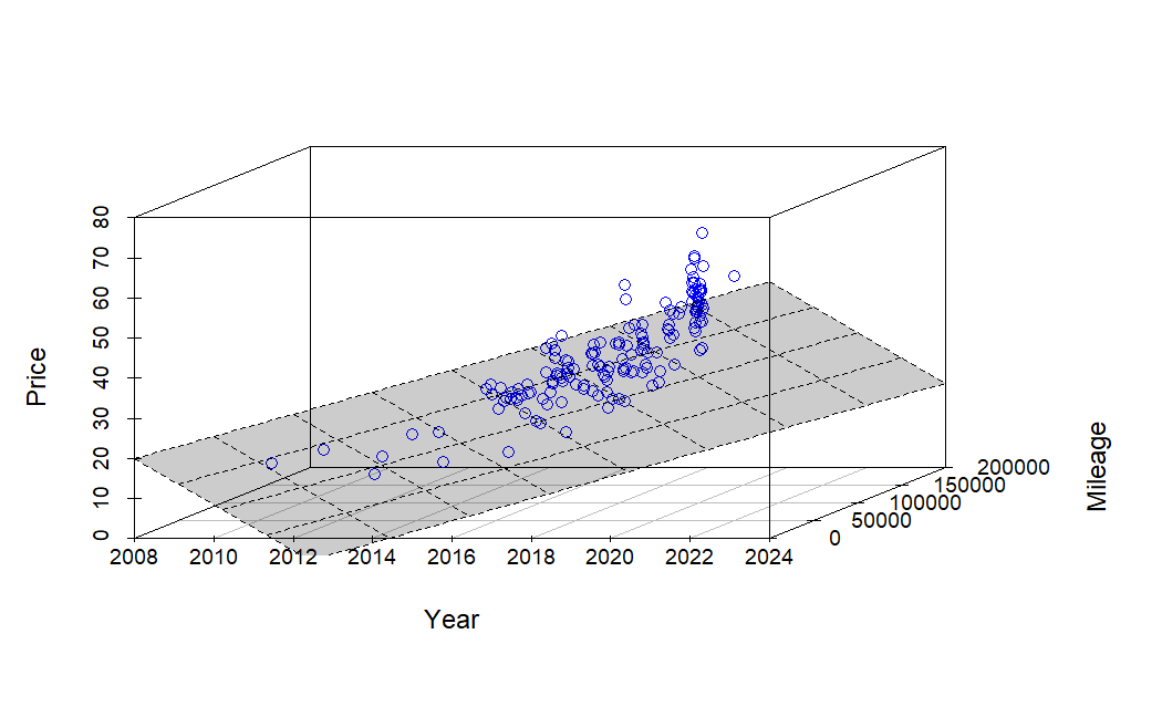
I built a much better model with more realistic constraints available here

Outside of generating new information or product, risk, diversity and time horizon are only variables I’m convinced an investor can control. This means invest broadly over long time horizons and keep taxes and expenses low. If you want outsized returns, you must take on more risk or make something people want to buy. Most wealth is created by businesses making real products, but wealth can still accumulate from appreciating assets (real estate, land, gold, internet domain names, etc). However, both these methods take a lot of time and effort. Can you make a lot more quickly through selling VOIP services, posting internet ads and joining a Brazilian-focused multi-level marketing (MLM) club called TelexFree?

Continue reading “TelexFree — A quick business case assessment”