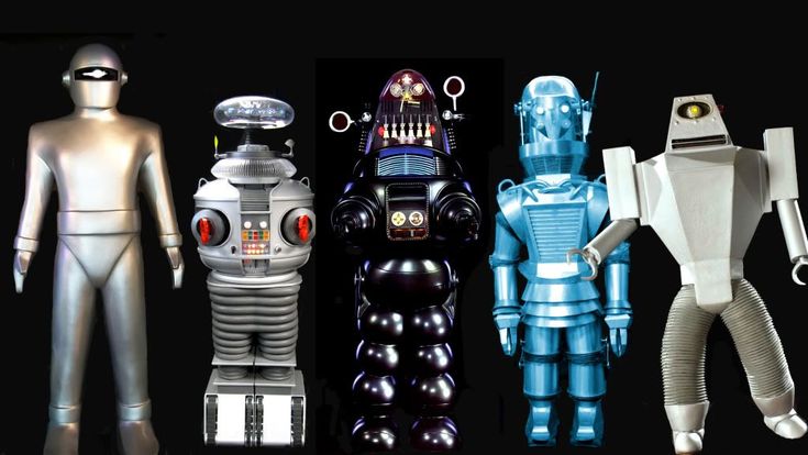
All those wireless Mice! (from Taiwan)

If you are like us, you get too many mice and keyboards lying around. With 5 or six devices, and an equal number of receivers you can just plug stuff in to find what matches. That assumes the peripherals are working and haven’t been lost. Can we interrogate the usb receivers and discover their associated hardware?

First, the findings: I tried four random USB receivers and found out their purpose and matching peripherals (Amazon Basics and Logitech) via windows powershell commands I share below. The interesting thing is that each one was made by a different company from the North part of Taiwan. These are huge companies that I’ve never heard of, each taking parts from the TSMC ecosystem and putting them into devices. The Amazon Basics companies were Pixart Imaging, Inc, MOSART Semiconductor Corporation and Chicony Electronics.

Pixart Imaging, Inc

If you want to follow the tech details below, I’m eager to show how I figured out what these black boxes are for the three different receivers.

All three of these companies were close to each other on the north side of Taiwan.

What are the numbers that identify these receivers?

First, some background. Each device has a ClassGuid, a unique identifier assigned to a device class in the Windows operating system. A device class is a group of devices that have similar characteristics and perform similar functions. The ClassGuid provides a way for Windows to recognize and manage different types of devices connected to the system.

You look into something small like this, the well goes deep. The logitech part had external serial numbers and government spectrum identifiers, the Amazon Basics parts required me to use windows PowerShell to learn about them.

The ClassGuid was originally defined by the Open Software Foundation (OSF) as part of the Distributed Computing Environment (DCE).

Today, the UUID specification is maintained by the Internet Engineering Task Force (IETF) as part of the Request for Comments (RFC) series. The current UUID specification can be found in RFC 4122, titled “A Universally Unique IDentifier (UUID) URN Namespace.”

RFC 4122 defines the structure and generation algorithms for UUIDs, ensuring that the generated identifiers are unique across different systems and over time. It covers various UUID versions that use different methods for generating unique values, such as time-based, random-based, or name-based algorithms.

Each device class in Windows has its own ClassGuid, which is typically a hexadecimal string enclosed in braces (e.g. {4d36e967-e325-11ce-bfc1-08002be10318}). The ClassGuid is used to associate a device driver with the corresponding device class, allowing the operating system to communicate with the device and perform necessary functions.

For example, when you connect a USB device to your computer, Windows uses the ClassGuid to determine which driver to use to communicate with the device. If the device is a Human Interface Device (HID), such as a mouse or keyboard, Windows will use the HID driver associated with the {745a17a0-74d3-11d0-b6fe-00a0c90f57da} ClassGuid. If the device is a USB mass storage device, Windows will use the storage driver associated with the {4d36e967-e325-11ce-bfc1-08002be10318} ClassGuid.

The ClassGuid for USB receivers, or USB dongles, will depend on the type of device.

For example, if you have a USB Wi-Fi adapter or a Bluetooth dongle, their ClassGuids will be either:

  • USB Wi-Fi adapter: {4d36e972-e325-11ce-bfc1-08002be10318} (Network adapters)
  • Bluetooth dongle: {e0cbf06c-cd8b-4647-bb8a-263b43f0f974} (Bluetooth radios)

However, if you have a USB receiver for a wireless mouse or keyboard, its ClassGuid will be that of a Human Interface Device (HID), which is {745a17a0-74d3-11d0-b6fe-00a0c90f57da}.

First Dongle, by Logitech

First, you can look at the device and read a couple numbers (only by taking pictures with my iPhone and zooming in, then using their character recognition).

Looking at the outside I see FCC ID JNZCU0010 refers to a specific device authorized by the Federal Communications Commission (FCC) in the United States. The FCC ID is an alphanumeric code that is assigned to devices that have been tested and comply with the FCC’s requirements for radio frequency interference, safety, and other regulatory standards.

The FCC ID JNZCU0010 belongs to the Logitech Unifying Receiver, which is a wireless USB receiver that connects multiple compatible Logitech devices, such as keyboards and mice, to a single computer using a 2.4 GHz wireless connection. This receiver is particularly useful for reducing the number of USB ports occupied by input devices and for providing a seamless connection experience between compatible Logitech peripherals.

You can find more information about the device by searching the FCC’s equipment authorization database with the FCC ID. The database typically contains documents related to the device’s testing, internal and external photos, and user manuals. You can access the database here: https://www.fcc.gov/oet/ea/fccid

The “IC” code, in this case, “IC: 4418A-CU0010”, refers to an Industry Canada (IC) certification number for the device. Industry Canada is the Canadian government agency responsible for regulating and certifying radio frequency devices, ensuring that they meet the necessary requirements and do not cause harmful interference.

Similar to the FCC ID in the United States, the IC certification number identifies a specific device tested and approved for use in Canada. The IC number “4418A-CU0010” is associated with the same Logitech Unifying Receiver that the FCC ID JNZCU0010 refers to.

So, both the FCC ID JNZCU0010 and the IC number 4418A-CU0010 identify the Logitech Unifying Receiver, confirming that it has been tested and certified for use in both the United States and Canada. This is enough to learn all I need about this receiver. A quick Bing/Google can tell you it’s compatible with: It is compatible with all Logitech Unifying products, which include mice and keyboards that have a Unifying logo displayed on them. You can connect up to 6 compatible keyboards and mice to one computer with a single Unifying receiver.

Active Interrogation for the unmarked receivers

While I’m a linux user, I’ve learned a bit of Windows PowerShell since that is where the hardware is directly connected. Let’s use windows to find out about the black boxes that have no markings that Amazon uses. Hint, it’s going to take us into the crazy Taiwanese CMOS ecosystem.

This command uses the “Get-PnpDevice” cmdlet to get a list of all the Plug and Play (PnP) devices currently connected to your computer. The “-PresentOnly” parameter limits the results to only devices that are currently connected. The “Where-Object” cmdlet is then used to filter the results to only devices with a ClassGuid that begins with ‘{‘, which is the format of all ClassGuids.

The “Select-Object” cmdlet is used to select the “ClassGuid”, “FriendlyName”, “Manufacturer”, “Description”, and “DeviceID” properties of each device. The “-Unique” parameter ensures that each device is only listed once.

When you run this command, you will see a list of all the ClassGuids associated with their respective devices. The output will include the device’s FriendlyName, which is a human-readable name for the device; the Manufacturer, which is the company that produced the device; the Description, which is a brief description of the device’s function; and the DeviceID, which is a unique identifier for the device. This additional information should give you a better understanding of what each connected device is and what its purpose is.

You can paste these commands into powershell and learn a lot:

Get-PnpDevice -PresentOnly | Where-Object {$_.ClassGuid -like '{*}'} | Select-Object ClassGuid, FriendlyName, Manufacturer, Description, DeviceID -Unique

or to find what we are looking for:

Get-PnpDevice -PresentOnly | Where-Object {($_.ClassGuid -eq '{745a17a0-74d3-11d0-b6fe-00a0c90f57da}') -or ($_.ClassGuid -eq '{4d36e96f-e325-11ce-bfc1-08002be10318}' -and $_.Description -like '*USB Receiver*')} | Select-Object ClassGuid, FriendlyName, Manufacturer, Description, DeviceID -Unique

This command queries Win32_USBControllerDevice for USB devices, and then retrieves detailed information on each device. The output will display the PNPDeviceID and the Description for each USB device.

You can then check the output for the relevant device and see if the model number (CU0010) is mentioned in the device description or the PNPDeviceID. If the model number is not explicitly mentioned, you might be able to find a unique identifier for the device that can help you confirm the model number through an online search or by checking the device documentation.

So if we run:

Get-WmiObject Win32_USBControllerDevice -Impersonation Impersonate | Foreach-Object { [Wmi]$_.Dependent } | Select-Object PNPDeviceID, Description

So I plug in a mystery receiver (bad idea) and that produces this output on my machine. Note the VID (vendor id) and PID (part id). You can look up parts based on that.

USB\VID_3938&PID_1059\6&208E681&0&3                USB Composite Device
USB\VID_3938&PID_1059&MI_00\7&E30261B&0&0000       USB Input Device
HID\VID_3938&PID_1059&MI_00\8&3483BAC7&0&0000      HID Keyboard Device
USB\VID_3938&PID_1059&MI_01\7&E30261B&0&0001       USB Input Device
HID\VID_3938&PID_1059&MI_01&COL01\8&C190CFE&0&0000 HID-compliant mouse
HID\VID_3938&PID_1059&MI_01&COL02\8&C190CFE&0&0001 HID-compliant consumer control device
HID\VID_3938&PID_1059&MI_01&COL03\8&C190CFE&0&0002 HID-compliant system controller
HID\VID_3938&PID_1059&MI_01&COL04\8&C190CFE&0&0003 HID-compliant vendor-defined device
HID\VID_3938&PID_1059&MI_01&COL05\8&C190CFE&0&0004 HID-compliant device

The  USB Implementers Forum (USB-IF) assigns vendor ID 3938 to MOSART Semiconductor Corporation, a Taiwan-based company that designs and develops integrated circuits (ICs) such as consumer ICs, PC peripheral ICs, and wireless consumer ICs.

Through some googling, I can find ou this is connected to my amazon basics keyboard:

KeyValue
BrandAmazon Basics
Item model numberKS1-US
Operating SystemWindows 7
Item Weight1.05 pounds
Product Dimensions5.61 x 1.13 x 17.83 inches
Item Dimensions LxWxH5.61 x 1.13 x 17.83 inches
ColorBlack
Batteries2 AAA batteries required. (included)
ManufacturerAmazon Basics
ASINB07WV5WN7B
Country of OriginChina
Date First AvailableNovember 11, 2019
Product Details

It’s strange that most components are made in Taiwan, but Country of Origin is listed as China.

A random dongle

Let’s try the next one, I connect a usb receiver with absolutely zero markings on it and find:

USB\VID_04F2&PID_1825\6&208E681&0&4           USB Input Device
HID\VID_04F2&PID_1825&COL01\7&295CC939&0&0000 HID-compliant mouse
HID\VID_04F2&PID_1825&COL02\7&295CC939&0&0001 HID-compliant vendor-defined device

The new device appears to be a USB Input Device with VID (Vendor ID) “04F2” and PID (Product ID) “1825”. VID “04F2” belongs to Chicony Electronics, a company that manufactures computer peripherals such as keyboards and mice. So where is  群光電子股份有限公司 located?

Just another 50 story building in a far away place.

In this case, the USB Input Device seems to be a multi-function device, as it includes both an HID-compliant mouse and an HID-compliant vendor-defined device. The device might be a mouse with additional features or a keyboard with an integrated touchpad. I had to set it aside and marvel and the world’s CMOS supply chain.

Trying my last device:

USB\VID_093A&PID_2510\5&7993A9C&0&2 - USB Input Device
HID\VID_093A&PID_2510&COL01\6&5B1E42D&1&0000 - HID-compliant mouse
HID\VID_093A&PID_2510&COL02\6&5B1E42D&1&0001 - HID-compliant vendor-defined device
HID\VID_093A&PID_2510&COL03\6&5B1E42D&1&0002 - HID-compliant consumer control device
HID\VID_093A&PID_2510&COL04\6&5B1E42D&1&0003 - HID-compliant system controller

So the vendor ID is Pixart Imaging, Inc and the part number is for an “optical mouse”.

is a Taiwan-based company founded in 1998 that specializes in designing and manufacturing CMOS (Complementary Metal-Oxide-Semiconductor) image sensors and related imaging application products. These components are commonly used in various devices, such as optical mice, digital cameras, webcams, and other consumer electronics.

One of the key products that Pixart Imaging is known for is its optical navigation sensors used in computer mice. These sensors replaced traditional mechanical ball-tracking mechanisms, allowing for more accurate and responsive cursor movement. The company’s optical sensors are widely used by different mouse manufacturers due to their high performance, low power consumption, and cost-effectiveness.

In addition to optical sensors, Pixart Imaging also offers a range of other products, such as capacitive touch controllers, fingerprint identification modules, and gesture recognition solutions. These components are utilized in a variety of applications, including smartphones, tablets, wearables, and IoT devices.

What are each of these entries?

  1. USB\VID_093A&PID_2510\5&7993A9C&0&2 – USB Input Device: This is a generic USB input device that can be used to transmit data between the connected device and the computer. It could represent a variety of peripherals, such as keyboards or game controllers.
  2. HID\VID_093A&PID_2510&COL01\6&5B1E42D&1&0000 – HID-compliant mouse: This entry represents a Human Interface Device (HID) compliant mouse. It follows the HID protocol to communicate with the computer, allowing for plug-and-play functionality and seamless interaction between the user and the computer.
  3. HID\VID_093A&PID_2510&COL02\6&5B1E42D&1&0001 – HID-compliant vendor-defined device: This entry represents a device that adheres to the HID protocol, but its specific function is defined by the vendor. It could be a custom input device or a specialized peripheral designed for a particular purpose.
  4. HID\VID_093A&PID_2510&COL03\6&5B1E42D&1&0002 – HID-compliant consumer control device: This is a Human Interface Device that is specifically designed for consumer electronics control, such as multimedia keyboards, remote controls, or other devices used to control media playback or volume.
  5. HID\VID_093A&PID_2510&COL04\6&5B1E42D&1&0003 – HID-compliant system controller: This entry represents a device that follows the HID protocol and serves as a system controller. It could be a device like a power management controller, system monitoring device, or another type of controller that helps manage various aspects of a computer system.

So, I was able to quickly find out this matched my Amazon Basics Mouse.

Time to catch my flight.

Quick(ish) Price Check on a Car

So, is it a good price?

With my oldest daughter heading off to college soon, we’ve realized that our family car doesn’t need to be as large as it used to be. We’ve had a great relationship with our local CarMax over the years, and we appreciate their no-haggle pricing model. My wife had her eyes set on a particular model: a 2019 Volvo XC90 T6 Momentum. The specific car she found was listed at $35,998, with 47,000 miles on the odometer.

But is the price good or bad? As a hacker/data scientist, I knew could get the data to make an informed decision but doing analysis at home is a great way to learn and use new technologies. The bottom line is that the predicted price would be $40,636 or 11.4% higher than the CarMax asking price. If I compare to the specific trim, the price should be $38,666. So the price is probably fair. Now how did I come up with that number?

Calculations

Armed with Python and an array of web scraping tools, I embarked on a mission to collect data that would help me determine a fair value for our new car. I wrote a series of scripts to extract relevant information, such as price, age, and cost from various websites. This required a significant amount of Python work to convert the HTML data into a format that could be analyzed effectively.

Once I had amassed a good enough dataset (close to 200 cars), I began comparing different statistical techniques to find the most accurate pricing model. In this blog post, I’ll detail my journey through the world of logistic regression and compare it to more modern data science methods, revealing which technique ultimately led us to the fairest car price.

First, I did some basic web searching. According to Edmunds, the average price for a 2019 Volvo XC90 T6 Momentum with similar mileage is between $33,995 and $43,998 and my $35,998 falls within this range.

As for how the Momentum compares to other Volvo options and similar cars, there are a few things to consider. The Momentum is one of four trim levels available for the 2019 XC902. It comes with a number of standard features, including leather upholstery, a panoramic sunroof, and a 9-inch touchscreen infotainment system. Other trim levels offer additional features and options.

The 2019 Volvo XC90 comes in four trim levels: Momentum, R-Design, Inscription, and Excellence. The R-Design offers a sportier look and feel, while the Inscription adds more luxury features. The Excellence is the most luxurious and expensive option, with seating for four instead of seven. The Momentum is the most basic.

In terms of similar cars, some options to consider might include the Audi Q7 or the BMW X5. Both of these SUVs are similarly sized and priced to the XC90.

To get there, I had to do some web scraping, data cleaning, and built a basic logistic regression model, as well as other modern data science methods. To begin my data collection journey, I decided (in 2 seconds) to focus on three primary sources: Google’s search summary, Carvana, and Edmunds.

My first step was to search for Volvo XC90 on each of these websites. I then used the Google Chrome toolbar to inspect the webpage’s HTML structure and identify the <div> element containing the desired data. By clicking through the pages, I was able to copy the relevant HTML and put this in a text file, enclosed within <html> and <body> tags. This format made it easier for me to work with the BeautifulSoup Python library, which allowed me to extract the data I needed and convert it into CSV files.

Since the data from each source varied, I had to run several regular expressions on many fields to further refine the information I collected. This process ensured that the data was clean and consistent, making it suitable for my upcoming analysis.

Finally, I combined all the data from the three sources into a single CSV file. This master dataset provided a solid foundation for my pricing analysis and allowed me to compare various data science techniques in order to determine the most accurate and fair price for the 2019 Volvo XC90 T6 Momentum.

In the following sections, I’ll delve deeper into the data analysis process and discuss the different statistical methods I employed to make our car-buying decision.

First, data from carvana looked like this:

<div class="tk-pane full-width">
    <div class="inventory-type carvana-certified" data-qa="inventory-type">Carvana Certified
    </div>
    <div class="make-model" data-qa="make-model">
        <div class="year-make">2020 Volvo XC90</div>
    </div>
    <div class="trim-mileage" data-qa="trim-mileage"><span>T6 Momentum</span> • <span>36,614
            miles</span></div>
</div>
<div class="tk-pane middle-frame-pane">
    <div class="flex flex-col h-full justify-end" data-qa="pricing">
        <div data-qa="price" class="flex items-end font-bold mb-4 text-2xl">$44,990</div>
    </div>
</div>

In this code snippet, I used the BeautifulSoup library to extract relevant data from the saved HTML file, which contained information on Volvo XC90 listings. The script below searches for specific <div> elements containing the year, make, trim, mileage, and price details. It then cleans up the data by removing unnecessary whitespace and commas before storing it in a dictionary. Finally, the script compiles all the dictionaries into a list and exports the data to a CSV file for further analysis.

I could then repeat this process with Google to get a variety of local sources.

One challenge from the Google results, was that I had a lot of data in the images (they were base64 encoded) so wrote a bash script to clean up the tags using sed (pro tip: learn awk and sed)

When working with the Google search results, I had to take a slightly different approach compared to the strategies used for Carvana and Edmunds. Google results did not have a consistent HTML structure that could be easily parsed to extract the desired information. Instead, I focused on identifying patterns within the text format itself to retrieve the necessary details. By leveraging regular expressions, I was able to pinpoint and extract the specific pieces of information, such as the year, make, trim, mileage, and price, directly from the text. My scrape code is below.

Scraping Edmunds required both approaches of using formatting and structure.

All together, I got 174 records of used Volvo XC90s, I could easily get 10x this since the scripts exist and I could mine craigslist and other places. With the data I have, I can use R to explore the data:

# Load the readxl package
library(readxl)
library(scales)
library(scatterplot3d)

# Read the data from data.xlsx into a data frame
df <- read_excel("data.xlsx")

df$Price<-as.numeric(df$Price)/1000

# Select the columns you want to use
df <- df[, c("Title", "Desc", "Mileage", "Price", "Year", "Source")]

# Plot Year vs. Price with labeled axes and formatted y-axis
plot(df$Year, df$Price, xlab = "Year", ylab = "Price ($ '000)",
     yaxt = "n")  # Don't plot y-axis yet

# Add horizontal grid lines
grid()

# Format y-axis as currency
axis(side = 2, at = pretty(df$Price), labels = dollar(pretty(df$Price)))

abline(lm(Price ~ Year, data = df), col = "red")
Armed with this data, we can assign a logistic regression model.

This code snippet employs the scatterplot3d() function to show a 3D scatter plot that displays the relationship between three variables in the dataset. Additionally, the lm() function is utilized to fit a linear regression model, which helps to identify trends and patterns within the data. To enhance the plot and provide a clearer representation of the fitted model, the plane3d() function is used to add a plane that represents the linear regression model within the 3D scatter plot.

model <- lm(Price ~ Year + Mileage, data = df)

# Plot the data and model
s3d <- scatterplot3d(df$Year, df$Mileage, df$Price,
                     xlab = "Year", ylab = "Mileage", zlab = "Price",
                     color = "blue")
s3d$plane3d(model, draw_polygon = TRUE)

So, we can now predict the price of 2019 Volvo XC90 T6 Momentum with 47K miles, which is $40,636 or 11.4% higher than the CarMax asking price of $35,998.

# Create a new data frame with the values for the independent variables
new_data <- data.frame(Year = 2019, Mileage = 45000)

# Use the model to predict the price of a 2019 car with 45000 miles
predicted_price <- predict(model, new_data)

# Print the predicted price
print(predicted_price)

Other Methods

Ok, so now let’s use “data science”. Besides linear regression, there are several other techniques that I can use to take into account the multiple variables (year, mileage, price) in your dataset. Here are some popular techniques:

Decision Trees: A decision tree is a tree-like model that uses a flowchart-like structure to make decisions based on the input features. It is a popular method for both classification and regression problems, and it can handle both categorical and numerical data.

Random Forest: Random forest is an ensemble learning technique that combines multiple decision trees to make predictions. It can handle both regression and classification problems and can handle missing data and noisy data.

Support Vector Machines (SVM): SVM is a powerful machine learning algorithm that can be used for both classification and regression problems. It works by finding the best hyperplane that separates the data into different classes or groups based on the input features.

Neural Networks: Neural networks are a class of machine learning algorithms that are inspired by the structure and function of the human brain. They are powerful models that can handle both numerical and categorical data and can be used for both regression and classification problems.

Gradient Boosting: Gradient boosting is a technique that combines multiple weak models to create a stronger one. It works by iteratively adding weak models to a strong model, with each model focusing on the errors made by the previous model.

All of these techniques can take multiple variables into account, and each has its strengths and weaknesses. The choice of which technique to use will depend on the specific nature of your problem and your data. It is often a good idea to try several techniques and compare their performance to see which one works best for your data.

I’m going to use random forest and a decision tree model.

Random Forest

# Load the randomForest package
library(randomForest)

# "Title", "Desc", "Mileage", "Price", "Year", "Source"

# Split the data into training and testing sets
set.seed(123)  # For reproducibility
train_index <- sample(1:nrow(df), size = 0.7 * nrow(df))
train_data <- df[train_index, ]
test_data <- df[-train_index, ]

# Fit a random forest model
model <- randomForest(Price ~ Year + Mileage, data = train_data, ntree = 500)

# Predict the prices for the test data
predictions <- predict(model, test_data)

# Calculate the mean squared error of the predictions
mse <- mean((test_data$Price - predictions)^2)

# Print the mean squared error
cat("Mean Squared Error:", mse)

The output from the random forest model you provided indicates that the model has a mean squared error (MSE) of 17.14768 and a variance explained of 88.61%. A lower MSE value indicates a better fit of the model to the data, while a higher variance explained value indicates that the model can explain a larger portion of the variation in the target variable.

Overall, an MSE of 17.14768 is reasonably low and suggests that the model has a good fit to the training data. A variance explained of 88.61% suggests that the model is able to explain a large portion of the variation in the target variable, which is also a good sign.

However, the random forest method shows a predicted cost of $37,276.54.

I also tried cross-validation techniques to get a better understanding of the model’s overall performance (MSE 33.890). Changing to a new technique such as a decision tree model, turned MSE into 50.91. Logistic regression works just fine.

Adding the Trim

However, I was worried that I was comparing the Momentum to the higher trim options. So to get the trim, I tried the following prompt in Gpt4 to translate the text to one of the four trims.

don't tell me the steps, just do it and show me the results.
given this list add, a column (via csv) that categorizes each one into only five categories Momentum, R-Design, Inscription, Excellence, or Unknown

That worked perfectly and we can see that we have mostly Momentums.

ExcellenceInscriptionMomentumR-DesignUnknown
Count0688789
Percent0.00%39.53%50.58%4.65%5.23%
Frequency and Count of Cars

And this probably invalidates my analysis as Inscriptions (in blue) do have clearly higher prices:

Plot of Price By Year

We can see the average prices (in thousands). In 2019 Inscriptions cost less than Momentums? That is probably a small n problems since we only have 7 Inscriptions and 16 Momentum’s in our data set for 2019.

YearR-DesignInscriptionMomentum
2014$19.99NANA
2016$30.59$32.59$28.60
2017$32.79$32.97$31.22
2018$37.99$40.69$33.23
2019NA$36.79$39.09
2020NA$47.94$43.16
Average Prices by Trim (in thousand dollars)

So, if we restrict our data set smaller, what would the predicted price of the 2019 Momentum be? Just adding a filter and running our regression code above we have $38,666 which means we still have a good/reasonable price.

Quick Excursion

One last thing I’m interested in: does mileage or age matter more. Let’s build a new model.

# Create Age variable
df$Age <- 2023 - df$Year

# Fit a linear regression model
model <- lm(Price ~ Mileage + Age, data = df)

# Print the coefficients
summary(model)$coef
EstimateStd. Errort valuePr(>|t|)
(Intercept)61.349130.6908488.803722.28E-144
Mileage-0.000222.44E-05-8.838691.18E-15
Age-2.754590.27132-10.15253.15E-19
Impact of Different Variables

Based on the regression results, we can see that both Age and Mileage have a significant effect on Price, as their p-values are very small (<0.05). However, we can also see that Age has a larger absolute t-score (-10.15) than Mileage (-8.84), indicating that Age may have a slightly greater effect on Price than Mileage. Additionally, the estimates show that for every one-year increase in Age, the Price decreases by approximately 2.75 thousand dollars, while for every one-mile increase in Mileage, the Price decreases by approximately 0.0002 thousand dollars (or 20 cents). That is actually pretty interesting.

This isn’t that far off. According to the US government, a car depreciates by an average of $0.17 per mile driven. This is based on a five-year ownership period, during which time a car is expected to be driven approximately 12,000 miles per year, for a total of 60,000 miles.

In terms of depreciation per year, it can vary depending on factors such as make and model of the car, age, and condition. However, a general rule of thumb is that a car can lose anywhere from 15% to 25% of its value in the first year, and then between 5% and 15% per year after that. So on average, a car might depreciate by about 10% per year.

Code

While initially in the original blog post, I moved all the code to the end.

Carvana Scrape Code

Cleaner Code

Google Scrape Code

Edumund’s Scrape Code

Autoscoring with Matlab

While I qualified a long time ago on the M9, I never really learned to be a good shot. Now, I’m trying to learn to shoot well and wanted to automatically score my targets, keep the data, and get better.

There are apps to do this, but none of them did what I wanted. One app by Thomas Gabrowski and Justa Mili works off a photo of the target to automatically calculate the score. They also have the capability to analyze shooting groups with Windage, Elevation, Mean Radius and Extreme Spread. They have capabilities to keep track of your previous shooting sessions and monitor progress. The App costs $17.

Developing my own costs my time, but gives me flexibility to work with my targets and my system. It’s also a thing I do: grab challenges that will teach me something. It’s served me well and Matlab makes this all accessible and fun. The other thing is that apps never work exactly right. What if I want the raw data so I can calculate if I’m aiming high or low over time? All this code is on github at https://github.com/tbbooher/automatic_target_scoring.

I told my children that two key skills every digital citizen needs are the ability to process text and images. By processing text, I’m able to tell any story from any reports in digital form. This is often bank statements, hotel stays, fitness stuff or uber rides. By processing images, I’m able to understand and report on things that are happening around me.

In looking around, I found this thesis filled with some good ideas. I reached out to the author and discussed the merits of edge detection vs template matching. He didn’t have his code available. There were several papers but none were really that helpful. It was easier to start building than to spend a lot of time reading other’s approaches.

I knew there would be three steps to this: (1) registering all images to the standard, fixed, image for consistent distance, (2) finding the bullet holes/center and (3) measuring the distances from the center each hole.

Image Registration

This was harder than I thought since most registration is for two similar images. I was used to the ease of Photoshop for rapid registration. It turns out it is a hard problem to register images of different pictures of what are really different scenes, even though the structure is common. Most image registration problems are pictures of the same scene that have been taken at different angles or distances. The picture below makes this clear:

Reference and Real Image

I found two approaches that worked for image registration. The first approach was to extract the red circle and then make the circles match. Here I had to calculate and align the centers, and rescale one image to the size of the other. Color thresholding and imfindcircle were quite useful.

For the more general case, I had to use fitgeotrans which takes the pairs of control points, movingPoints and fixedPoints, and uses them to infer the geometric transformation. It does this by taking the pairs of control points, movingPoints and fixedPoints, and uses them to infer the geometric transformation. After doing this I had a set of images that were all the same size, and all in the same orientation — with bullet holes.

Registered Images

Finding the bullet holes

I was able to use this matlab post to learn that I could sample some colors in photoshop, convert the image to HSV and find shades of gray using some code from Theodoros Giannakopoulos.

The next thing I had to do was create the ability to find the center. I did this by recognizing that the center X is red and pretty distinctive — ideal for template matching using normalized cross-correlation matlab has a great description of how this works here. With this accomplished, I can find the center in a few lines, by going off this template:

Template

All together, I’m able to compute the measurements to make a picture like this (note the green circle in the middle on the X):

Result

With the image registered, the center defined and all holes discovered, I could easily calculate a score of a mean distance to the bullseye.

Problems

The problem was that I couldn’t get good consistency. The shadows were a problem on some images, on others, shots very close to one another caused confusion. It turned out that I was really good at quickly seeing the holes, better than a template matching problem. Note that when I saved the image, I updated a xls file and saved the scores as EXIF data so the image had the exact locations of the holes that I could pull out later if needed. The code below works awesome and is ideal for my solution. Best of all, I learned a lot about how to manipulate and extract data from images.

Results

So, is my shooting getting better? Not yet. In the plot below you can see my score is increasing, and the stDev of my shots is increasing as well. Now, the data aren’t uniform since I had the target at 5m and now have it at 6.5m on Oct 8. Sept 12 was with a suppressed 22 at 5m. Oct 8 was 9mm. Anyway, it’s better to know from data than to be guessing. I’m chalking this up to an improved technique that is taking some time to adjust to.

Nginx With Https for Local Development

Testing HTTPs locally is always hard, but I’m against testing on production or even on a remote server.
Things are also complicated by developing in linux as a subsystem on windows via WSL2. I was able to use mkcert to get ssl to work locally.
While I would love to use Let’s Encrypt locally, Let’s Encrypt can’t provide certificates for “localhost” because nobody uniquely owns it. Because of this, they recommend you generate your own certificate, either self-signed or signed by a local root, and trust it in your operating system’s trust store. Then use that certificate in your local web server. They describe this well on their website.

Using certificates from real certificate authorities (CAs) for development can be dangerous or impossible (for hosts like example.test, localhost or 127.0.0.1), but self-signed certificates cause trust errors. Managing my own CA may be the best solution, but mkcert automatically creates and installs a local CA in the system root store, and generates locally-trusted certificates. I was able to modify my nginx.conf with the my container test environment and open the necessary ports in docker-compose (- 443:443) to get this working just fine.
You can see my working code here on a new git branch.

upstream flask-web {
server flask:5000;
}

upstream lochagus-web {
server lochagus:8080;
}

server {
listen 80;
listen [::]:80;

location / {
root /usr/share/nginx/html/;
try_files $uri /index.html;
}

charset utf-8;
source_charset utf-8;

location /flask {
include /etc/nginx/conf.d/headers.conf;
proxy_pass http://flask-web/;
}

location /lochagus {
include /etc/nginx/conf.d/headers.conf;
proxy_pass http://lochagus-web/;
}

}

server {
listen 443 ssl http2;
listen [::]:443 ssl http2;
server_name tim.test.org;

charset utf-8;
source_charset utf-8;

location / {
root /usr/share/nginx/html/;
try_files $uri /index.html;
}

location /flask {
include /etc/nginx/conf.d/headers.conf;
proxy_pass http://flask-web/;
}

location /lochagus {
include /etc/nginx/conf.d/headers.conf;
proxy_pass http://lochagus-web/;
}

ssl_certificate /etc/nginx/certs/tim.test.org.pem;
ssl_certificate_key /etc/nginx/certs/tim.test.org-key.pem;

}

Organize Images

I deleted and recovered a large number of photos (thanks foremost). However, a large number of images from a browser cache was messing up my photo library.

Who wants to keep 10,000 of these images stored on my harddrive?

I used the number of unique colors to filter them out via MATLAB.

As expected, if I plot this, I get a nice s-curve:

plot(sort(nonzeros(ucolors)))

Or, viewing this as a histogram

histogram(nonzeros(ucolors),100)

So I modified the script to move all images with unique color counts less than 4500 unique colors to a folder: potential bad

This worked perfectly and saved my whole Saturday.

DEFCON 25 Writeup

Nothing delivers the fear of missing out like DEFCON. So much to learn and so little time. Too busy hacking in the IOT village or catching up with old friends to sit in on the talks? Read below to find out what you missed in my talk writeups below. They are listed in chronological order, with some of the most interesting at the end of the document, so don’t give up too easily.

Overall, conference attendance was at a record 27,000 people, most of them non-technical fans of hacking culture. Major themes continued a previous trend of focus on IOT, Drones, and low-level tools and vulnerabilities. New additions this year were a focus on analog techniques to both vet and attack low-level hardware. Several talks leveraged the increased performance and lower cost of commercial software defined radios.

The largest media coverage was focused on vulnerabilities to voting machines and the ability to use cheap components to crack physical protections.

All speakers and talk abstracts are listed here and most presentations can be found on the DEFCON media server. In roughly a month, all of these talks will be available on YouTube.

DEFCON Capture the Flag

The Capture the Flag (CTF) competition was won by CMU’s PPP team coached by David Brumley. This team won the last three years of the competition and several before that as well, and a majority of the PPP team members were on the winning DARPA Cyber Grand Challenge team as part of David Brumley’s company For All Secure.

DARPA’s Dustin Fraze ran this year’s competition, which was specifically designed to thwart any attempts to start the competition with a head start from a cyber reasoning system such as those developed for the DARPA Cyber Grand Challenge. In order to do this, the organizers developed a radically new architecture with several challenging properties:

  • 9-bit bytes instead of 8-bits. This makes parsing the binary difficult. The byte length of the architecture of the system parsing a challenge does not match that in cLEMENCy. The start of a byte on both systems would only match every 9th byte.
  • It’s Middle Endian. Every other architecture stores values in memory in one of two ways: from most significant byte to least significant (Big Endian), or least significant to most significant (Little Endian). Rather than storing a value like 0x123456 as 12 34 56 or 56 34 12, Middle Endian stores it as 34 56 12.
  • Instructions have variable length opcodes. Instructions were anywhere from 18 to 54 bits, with opcodes being anywhere from 4 bits to 18 bits.

Thursday:

Porosity: A Decompiler For Blockchain-Based Smart Contracts Bytecode – Matt Suiche

With the knowledge that implementation is always the most common cryptographic weakness, Matt described how to decompile and comprehend Ethereum smart contracts. Ethereum is an open software platform based on blockchain technology that enables developers to build and deploy decentralized applications, in this case smart contracts. The hacks of these contracts have been popular due to flawed implementations. The 2016 DAO (Decentralized Autonomous Organization) theft or the recent Parity multisignature blockchain wallet compromise resulted because of poorly written Solidity code (contract-oriented, high-level language) that introduced vulnerabilities which hackers exploited to steal funds from other Ethereum users, not because of compromises of the underlying blockchain protocol or cryptographic weakness.

In his talk, Matt presented “Porosity,” the first decompiler that generates human-readable Solidity syntax smart contracts from any EVM bytecode. Because compiled smart contracts are all world visible on the Ethereum network, this tool enables all contracts to be reviewed at any time. Once reversed, the code can be scanned to check for susceptibility to new attacks or to ensure adherence to best practices.

You can read his paper here for more details.

See No Evil, Hear No Evil: Hacking Invisibly and Silently With Light and Sound – Matt Wixey

Matt Wixey showed how attackers creatively bypass modern security protections through leveraging light and/or sound, using off-the-shelf hardware. His talk covered C2 channels and exfiltration using light and near-ultrasonic sound, to disable and disrupt motion detectors; he demonstrated use of home-built laser microphones, a technique for catapulting drones into the air and overriding operator controls, jamming speech through the use of delayed auditory feedback, and demotivating malware analysts. Specifically, he demonstrated:

  • Using acoustic ultrasonic pulses to disrupt a drone and render the controller useless by characterizing and sending specific inputs to ultrasonic altimeters. He demonstrated this over a large area through a cluster of ultrasonic transducers.
  • He displayed a demonstration of a covert acoustical mesh network at 16-20KhZ using steganography to conceal the transmission (he played the acoustic attack signal inside seemingly normal audio).
  • He was able to open a computer application by shining infrared light into its ambient light sensor near the webcam which triggered activation of pre-installed malware
  • He played music from a smartphone into a speaker without Bluetooth and without wires connecting the two devices, by using infrared LEDs within close proximity
  • Matt also demonstrated the ability to shut off his TV, when the theme song of Gilmore Girls played in his apartment.

His talk is available here.

Friday:

The Brain’s Last Stand – Garry Kasparov

Kasparov discussed the ways humans and intelligent machines could work together. He described that AI will not destroy jobs, but will make new ones. He also talked about the respective contributions of machines and people. The general consensus of the crowd was that he succeeded in providing a keynote that was both funny and insightful.

Weaponizing the BBC Micro:Bit – Damien Cauquil

The BBC has produced a Micro:bit, a pocket-sized computer for education. Damien showed that the Micro:bit can be configured to sniff out keystrokes from a wireless keyboard, and even take control of a quadcopter drone. He demonstrated using publicly available software, and a Micro:bit, the ability to snoop on signals and get the input from a wireless keyboard using Bluetooth. He also attached a Micro:bit to a drone controller handset and used the resulting hardware to interfere with an airborne quadcopter’s control mechanisms and hijack its flight controls.

His slides are available.

Hacking Smart Contracts – Konstantinos Karagiannis

While the Ethereum cryptocurrency core system remains secure, there have been a number of hacks of the Ethereum system. The most famous attack was against an smart contracts wallet, called the Parity Ethereum client. The vulnerability allowed the hacker to exfiltrate funds from multi-signature wallets created with Parity clients 1.5 and later. Konstantinos described the hack as shockingly basic: “It turns out that the creator [of the wallet] left out a very important word,” Karagiannis said. “And that one little word was the word ‘internal.’ When you don’t make that declaration, the program will accept what are called messages from an external source. So because he left off that simple declaration, attackers were able to craft a very simple message that told the wallet, ‘Hey, you belong to me now.’ After that was done, they were then able to do an execute command that then told the wallet, ‘And, by the way, I’d like that money sent here.’ So it was a really simple two-stage attack that should not have happened.”

This was a case where white hat hackers were clear heroes. He described anonymous vigilantes calling themselves the White Hat Group intervened, who stole Ether out of wallets before the hackers could get to it. Later, this group transferred the Ether back to its owners, saving about $200 million.

See the slides here.

Open Source Safe Cracking Robots – Nathan Seidle

One of the most well-received talks was by Nathan Seidle, founder of SparkFun Electronics. He demonstrated an open source safe-cracking robot. Using an Arduino and 3D printing, the safe-cracking robot cost around $200 to build. It uses magnets to attach to the exterior of a safe and is super simple to run with only one button.

They accomplished this by determining one of the dials within 20 seconds by detecting the larger size of the correct indent. The other two dials couldn’t be measured directly, but they were helped by finding that most safes have a built in margin of error. This enabled them to dramatically reduce the number of potential combinations.

See the slides or watch a video from Wired magazine.

Next-Generation Tor Onion Services – Roger Dingledine

Roger argued that a tiny fraction of Tor traffic makes up what is often called the “dark web”. He introduced the concept of “Tor onion services” which let people run internet services such as websites inside the anonymous Tor network.

He discussed how mistakes in the original protocol are now being actively exploited by threat intelligence companies to build lists of onion services even when the service operators thought they would stay under the radar. To fix this, he presented a new and improved onion service design, which provides stronger security and better scalability. For example, they are migrating from 1024-bit RSA encryption keys to shorter but tougher-to-crack ED-25519 elliptic curve keys.

He predicts that soon anyone will be able to create their own corner of the internet that’s not just anonymous and untraceable, but entirely undiscoverable without an invite. In particular, the new design will both strengthen the cryptosystem and let administrators easily create fully secret darknet sites that can only be discovered by those who know a long string of random characters. This is especially important due to the arrival of a large number of darknet indexing and search services.

These services will work by changing the basic mechanism of service declaration. Instead of declaring their .onion address to hidden service directories, they’ll derive a unique cryptographic key from that address which is discreetly stored in Tor’s hidden service directories. Any Tor user looking for a certain hidden service can perform that same derivation to check the key and route themselves to the correct darknet site. But the hidden service directory can’t derive the .onion address from the key. This means there is no known way to discover an onion address.

Applications for this include the ability for a small group of collaborators to host files on a computer known only to them that no one else could ever find or access. Also present are mitigations against the techniques used by law enforcement to find and remove the silk road servers in 2014.

Slides are available.

How We Created the First SHA-1 Collision and What it means For Hash Security – Elie Bursztein

The SHA1 cryptographic hash function is critical for the many of the cryptographic and integrity verifications that enable our current state of internet security. For example, Git, the world’s most widely used system for managing software development among multiple people, relies on it for data integrity. The basic security property of hash values is that they uniquely represent a given input, when it is possible to break this property on demand, a cash collision occurs. This February, the first SHA-1 collision was announced. This collision combined with a clever use of the PDF format allowed attackers to forge PDF pairs that have identical SHA-1 hashes and yet display different content. In the talk, Elie made it clear how difficult this was to achieve. This attack is the result of over two years of intense research. It took 6500 CPU years and 110 GPU years of computations to find the collision.

They discussed the challenges faced from developing a meaningful payload, to scaling the computation to that massive scale, to solving unexpected cryptanalytic challenges. They were able to discuss positive aspects of the release and presented the next generation of hash functions and what the future of hash security holds.

For more information, refer to this article from the register. No slides were available.

Breaking the x86 Instruction Set – Christopher Domas

Chris demonstrated how page fault analysis and some creative search strategies can be used to exhaustively search the x86 instruction set and uncover new secrets. In particular, I was impressed by his use of page boundaries to determine lengths of unknown instructions. He disclosed new x86 hardware glitches, previously unknown machine instructions, ubiquitous software bugs, and flaws in enterprise hypervisors. He also released his “sandsifter” toolset, that allows users to audit – and break – your own processor.

While he discovered a large number of hidden instructions, I think the really interesting work resulting from this will be from exploits developed from unknown opcodes. For example, an attacker can use these to mask malicious behavior. They could throw off disassembly and jump targets to cause analysis tools to miss the real behavior.

What worries me most is that hardware bugs are foundational and manifest themselves in the dependent software stack. Additionally, these are difficult to find and fix. For example, he presented a ring 3 processor DoS that I think would be difficult to counter.

They used these techniques to find innumerable bugs in disassemblers, the most interesting is a bug shared by nearly all disassemblers. Most disassemblers will parse certain jmp (e9) and call (e8) instructions incorrectly if they are prefixed with an operand size override prefix (66) in a 64 bit executable. In particular, IDA, QEMU, gdb, objdump, valgrind, Visual Studio, and Capstone were all observed to parse this instruction differently than it actually executes.

This is written up well in a (unpublished) paper here and the slides are available as well.

Abusing Certificate Transparency Logs – Hanno Böck

Hanno started by making the point that certificate transparency logs are not generally trusted by the information security community and highlighted several cases of illegitimate certificates in the past. However, he noted that there is no feasible plan how to replace CAs and in September 2017 Google will make Certificate Transparency mandatory for all new certificates and in the future logging will be required in April 2018. However, in practice, most certificates are currently logged and the certificate transparency system provides public logs of TLS certificates.

Certificate Transparency has helped uncover various incidents in the past where certificate authorities have violated rules. It is probably one of the most important security improvements that has ever happened in the certificate authority ecosystem.

While certificate transparency is primarily used to uncover security issues in certificates, Hanno Böck showed that these data are also valuable for other use cases to include attacks such as exploiting common web applications like WordPress, Joomla or Typo3 through exploiting certificate transparency.

  • Attack 1: Attacker monitors CT logs, extracts host names. Compares web pages with common installers.
  • Attack 2: Installer found: Install the application. Upload a plugin with code execution backdoor. Revert installation, leave backdoor.

Using the second attack, he claimed he could have taken over around 4000 WordPress installations within a month.

For more details, see this blog post and these slides.

Saturday:

On Saturday, I was surprised when 22 zero-day exploits were released against a range of consumer products—mainly home automation and Internet of Things devices.

A Picture is Worth a Thousand Words, Literally Deep Neural Networks for Social Stego – Philip Tully and Michael T. Raggo

Philip Tully and Michael T. Raggo described how steganography can be systematically automated and scaled. In order to accomplish this, they first characterized the distorting side effects rendered upon images uploaded to popular social network servers such as compression, resizing, format conversion, and metadata stripping. Then, they built a convolutional neural network that learned to reverse engineer these transformations by optimizing hidden data throughput capacity. They then used pre-uploaded and downloaded image files to teach the network to locate candidate pixels that are least modifiable during transit, allowing stored hidden payloads to be reliably recalled from newly presented images. Deep learning typically requires massive training data to avoid overfitting. However massive images are available through social networks’ free image hosting services, which feature bulk uploads and downloads of thousands of images at a time per album.

From this, they demonstrated the ability to show that hidden data can be predictably transmitted through social network images with high fidelity and low latency. This is significant, because steganalysis and other defensive forensic countermeasures are notoriously difficult, and their exfiltration techniques highlight the growing threat posed by automated, AI-powered red teaming.

The slides are available as is a good write-up.

MS Just Gave the Blue Team Tactical Nukes (And How Red Teams Need To Adapt) – Chris Thompson

This talk could presage the end of the nearly $2B endpoint security market on Windows (i.e. Symantec,Carbon Black, CrowdStrike, BigFix, CyberReason, FireEye).

Windows Defender Advanced Threat Protection (ATP) is a cloud-based data security service that provides advanced breach detection based on the information gathered by Microsoft’s massive threat intelligence system. This coming spring, it’s due for a big upgrade and Microsoft has used their knowledge of and deep access into the Windows operating system to give their tools unique capabilities, such as the inability to uninstall them via microsoft enterprise admin tools. (For example, it requires a generated offboarding script with a SHA256 signed reg key based on the unique Org ID and cert to uninstall).

I also found it interesting that the ATP sensor uses Windows Telemetry (DiagTrack service), which in turn uses WinHTTP Services (winhttp.dll.mui) to report sensor data and communicate with the Windows Defender ATP cloud service. Other interesting results in this talk were a demonstrated capability to perform Golden Tickets Detection (Using KRBTGT NTLM Hash), detecting malicious replication requests via DCSync and detection of internal recon activities.

The principal program manager of Windows Defender ATP at Microsoft was quoted as saying: “Windows Creators Update improves our OS memory and kernel sensors to enable detection of attackers who are employing in-memory and kernel-level attacks—shining a light into previously dark spaces where attackers hid from conventional detection tools. . . We’ve already successfully leveraged this new technology against zero-days attacks on Windows.”

Windows Defender ATP should definitely be carefully watched and tested going forward. Out of the box, it will provide at least a new layer of security, but it also has the potential to replace expensive EDR solutions.

This article is a good summary and the slides are available.

Trojan-tolerant Hardware & Supply Chain Security in Practice – Vasilios Mavroudis and Dan Cvrcek

Vasilios Mavroudis and Dan Cvrcek challenged the perception that high-assurance systems cannot tolerate the presence of compromised hardware components and demonstrate how trusted, high-assurance hardware can be built from untrusted and potentially malicious components.

They noted that the majority of IC vendors outsource the fabrication of their designs to facilities overseas, and rely on post-fabrication tests to weed out deficient chips. However they claim that these tests are not effective against: 1) subtle unintentional errors (e.g., malfunctioning RNGs) and 2) malicious circuitry (e.g., stealthy Hardware Trojans). These errors are very hard to detect and require constant upgrades of expensive forensics equipment, which contradicts the motives of fabrication outsourcing.

To meet this challenge, they introduced a high-level architecture that can tolerate multiple, malicious hardware components, and outlined a new approach in hardware compromise risk management. They contrasted this against existing approaches such as trusted foundries (very expensive, prone to errors), split-manufacturing (still expensive, not secure), post-fabrication inspection (expensive, a huge pain, doesn’t scale), secret-sharing (keys generated by a trusted party). By contrast, their system is a fault-tolerant computer system that runs the same set of operations at the same time in parallel and incorporates random number generation, key generation & management, decryption and signing. They claim this provides resilience and is tamper-resistant (FIPS-4).

Their implementation incorporated 120 SmartCards, quorums of three cards, 1.2Mbps dedicated inter-IC buses, ARTIX FPGA controls the communications bus and 1Gbit/s bandwidth for incoming requests. Their key innovation was using SmartCards

They benchmarked the performance of this system, and described its internals. They also quantified other techniques such as “component diversification” and “non-overlapping supply chains”, and finally discussed how “mutual distrust” can be exploited to further increase trust in hardware integrity.

The slides are available.

Evading next-gen AV using A.I. – Hyrum Anderson

With most next-generation antivirus solutions relying on machine learning to identify new iterations of malware, Hyrum used artificial intelligence to construct a system that would mutate malware to the point where it wouldn’t be detected while still keeping its form and function. Essentially, he created a test in which you could pit artificial intelligence against any next-generation antivirus solution where the artificial intelligence would manipulate the malware by modifying bytes (while preserving the malware) and test it against the antivirus solution to determine if it was identified as malicious or benign. Hyrum showed in his trials that this process was successful in modifying malware to bypass detection.

The slides are available.

Sunday:

Breaking Bitcoin Hardware Wallets – Josh Datko and Chris Quartier

In this talk Josh Datko and Chris Quartier explained that bitcoin security rests entirely in the security of one’s private key. Bitcoin hardware wallets (a separate device that stores your private key) help protect against software-based attacks to recover or misuse the private key. This talk explored how one could compromise the security of these hardware wallets. In 2015, Jochen Hoenicke was able to extract the private key from a TREZOR using a simple power analysis technique. While that vulnerability was patched, they explored the potential to exploit the Microcontroller on the TREZOR and the KeepKey. They accomplished this by using an Open Source Hardware tool, the Chip Whisperer. With this device, they tried to overview fault injection techniques, timing, and power analysis methods against the STM32F205 microcontroller on the Trezor and KeepKey.

The successful technique takes advantage of the properties of the power distribution networks on printed circuit boards to generate ringing in these networks. This ringing is presumed to perturb the power distribution networks on the target chip itself, which is known to cause faulty operations. The use of fine control over the fault timing has also demonstrated that faults with very high reliability can be inserted, determining for example if a single- or multi-bit fault should be introduced, or to fault a single byte out of a larger array operation. In general a glitch width of about 750 nS would frequently (50{aaa01f1184b23bc5204459599a780c2efd1a71f819cd2b338cab4b7a2f8e97d4} of the time) result in one or more bit flip in the register without noticeably damaging the FPGA design.

However, TREZOR (and all clones) did not enable Clock Security System in the MCU, allowing injection of clock faults and he wasn’t able to use the ability for these bit flips to compromise the keys on the device.

For more details, refer to the slides or this paper:

O’Flynn, Colin. “Fault Injection using Crowbars on Embedded Systems.” IACR Cryptology ePrint Archive 2016 (2016): 810.

Backdooring the Lottery, and Other Security Tales in Gaming over the Past 25 Years – Gus Fritschie and Evan Teitelman

In October 2015, Eddie Raymond Tipton, the information security director of the Multi-State Lottery Association (MUSL), was convicted of rigging a $14.3 million drawing of MUSL’s lottery game Hot Lotto. The trial found that Tipton had rigged the draw in question, by using his privileged access to a MUSL facility to install a rootkit on the computer containing Hot Lotto’s random number generator, and then attempting to claim a winning ticket with the rigged numbers anonymously. There is evidence that Eddie Tipton was able to steal a lot of other funds using similar techniques.

This worked by taking various game parameters including the number of numbers per draw and the maximum and minimum numbers in the game and multiplied them together along with the number 39 and the summed ASCII values of the letters in the computer name. Then he took that and added it to the day of the year and added in the product of the number of times the Pseudorandom number generator (PRNG) had run since the last reboot and the year. This number was then used to seed the PRNG. One of the clever things Tripton was able to do is ensure the certification would pass, even when they ran the output of the PRNG through statistical tests to ensure unbiased results.

The 2014 russian slot machine hack was also very interesting. Hackers reverse-engineered slot machine software and discovered a weakness in the PRNG. Their exploit against this weakness was to make a video of roughly 24 spins and to upload the resultant data to calculate the pattern based on the slots. This Information was transmitted to a custom app with a listing of timing marks that cause the mobile to vibrate 0.25 seconds before the spin button should be pressed. While this was not always successful, the result was a higher payout than expected. This is an excellent overview of this hack.

Their slides are interesting.

Genetic Diseases to Guide Digital Hacks of the Human Genome: How the Cancer Moonshot Program will Enable Almost Anyone to Crash the Operating System that Runs You or to End Civilization – John Sotos

John Sotos, the Chief Medical Officer at Intel, has a wild, scary thought experiment: What if, by investing in hacking the human genome for good, we’ve opened it up to be hacked for evil? He believes it may one day be possible to create terrifying bioweapons using genetics.

John claimed that the enabling capability for these attacks comes from data and techniques made available from the Human Genome Project and the Cancer Moonshot.

While mostly a thought experiment, John discussed the intersection between precise gene editing and digital biology (an emulative and bit accurate model of biological processes). From these, he claims it will be possible to digitally reprogram the human genome in a living human. In his mind, this raises the potential to give bio-hackers the ability to induce “deafness, blindness, night blindness, strong fishy body odor, total baldness, intractable diarrhea, massive weight gain, shouting involuntary obscenities, physical fragility, or a susceptibility to death from excitement. . .There are things worse than death”

No slides were available, but the press covered this talk extensively.

Revoke-Obfuscation: PowerShell Obfuscation Detection (And Evasion) Using Science – Daniel Bohannon and Lee Holmes

Delivery and execution of malware is often by basic malicious executables and malicious documents, but a small portion of the current malware ecosystem leverages PowerShell as part of its attack chain. Most commonly PowerShell calls an executable or document macro that launches PowerShell to download another executable and run it.

Many personal security products attempt to prevent this behavior, with two primary techniques: applying antivirus signatures to command line arguments and AMSI-based (Anti-malware Scan Interface) detection. But obfuscation and evasion techniques can bypass these protections. There is an inherent challenge to allowing powerful administrative behavior through an interface like powershell and preventing these tools from conducting malicious behavior.

While starting with numerous examples of how hard it is to block illicit use of PowerShell, this talk focused on how to detect invoke-obfuscation which can bypass both approaches. These advanced techniques leverage extreme levels of randomization in Invoke-Obfuscation and Invoke-CradleCrafter paired with the token-layer obfuscation options that are not deobfuscated in PowerShell’s script block logging. To counter these advanced techniques, they built a tool, called revoke-obfuscation, which uses statistical analysis to detect the most subtle obfuscation techniques. The heart of the technical capability is to use statistical tools to analyze the entropy and letter frequency distribution of the variable names.

One of the clever techniques they employ is to use cosine similarity to analyze the frequency of each letter in a script. However, this naive technique lacked the advantages of unsupervised approaches and statistical variance. Additionally, it was susceptible to character frequency tampering. To counter this, they downloaded 408,000 PowerShell scripts and modules. They then were able to apply logistic regression with gradient descent to calculate and summarize 4098 unique script characteristics to directly identify the likelihood that a script is obfuscated. Their results were fairly impressive with an accuracy and F1 score of 96{aaa01f1184b23bc5204459599a780c2efd1a71f819cd2b338cab4b7a2f8e97d4} and 95{aaa01f1184b23bc5204459599a780c2efd1a71f819cd2b338cab4b7a2f8e97d4}, respectively. This was 10 times better at finding obfuscated content than character frequency analysis alone, and has half of the false positives.

More details are available in this excellent report.

Common Mathmatical Libraries: Computation, History, and Trust

A common complaint among engineers is that modern computers obscure the details of the complicated math they produce. We cringe when children are exalted as “knowing computers” from a young age. Bill Gosper and Richard Greenblatt had perhaps the maximum benefit to “learn computers”. They didn’t have wolfram alpha or even spreadsheets, they had to understand arithmetic logic units and figure out how to optimize code to get basic math operations to run on the TRS-80. Today, there is a desire to re-learn hardware through arduino or other low-level hardware, but most folks start very high on the stack. That is a shame, because under the hood is a rich and exciting legacy of numerical computing software that forms the basis of the trust we place in computers.

My trust in computers started to erode when Mark Abramson gave a lecture on the possible errors of floating point arithmetic. All programmers are aware of the problems possible by a division by zero or a narrowing conversion that loses information. However, other times the cause can be the futile attempt of a software developer to round a floating-point number. This was shocking: one of the most basic operations in math, a thing that we learn to do before we can ride a bike, eludes the combined efforts of the finest engineers over the last 30 years. To me, this was something intuitively nonsensical: if computers can’t consistently and reliability round numbers, how can we trust them to do anything?

This turns out to be one of those things like the halting problem that proves it is impossible for a computer to understand computer code. Floating points are represented internally in the IEEE-754 specification. Just like the impossible realization of a random number1, there is no such thing as a true fractional number in a computer. The key thing is to recognize that floating types do not represent numbers exactly. Internally the value is not a continuous range of numbers; instead it is represented as an exponent multiplied by an arithmetical series. For example:

$$
\frac{1}{2}^1 + \frac{1}{2}^2 + \frac{1}{2}^3 + \ldots + \frac{1}{2}^{30}
$$

From the above, you can see that in any range of floating point numbers there are gaps. Between any two floating point numbers there is a difference at the granularity of the smallest element in the arithmetical series (here $\frac{1}{2}^{30}$). If a number falls in such a gap, the difference between the real number is the approximation error. This leads to a fascinating and esoteric subject, that is best covered by others.

In grad school, my faith in computers only decreased when I realized the challenges associated with Eigenvalue problems, Singular value decomposition and LU/Cholesky/QR/… decompositions. If you want to understand how these are handled, a rough understanding of high performance computing libraries is necessary. These libraries are important because of the issues described above. It is very important (and very hard) to have both an efficient and correct algorithm for matrix decomposition.

I spent my teens coding in BASIC, my college years in MATLAB, and professionally I’ve used lots of Julia, FORTRAN, Ruby, Python, C, Haskell, and x86 or MIPS assembly. As I’ve used different languages, I kept coming back to familiar libraries that every language used with strange names like LAPACK, BLAS, FFTW, and ATLAS.

MATLAB will always be the language that I call home. It is probably the only language I was paid at work to write production code with. In building and running large models, I had to get into the internals of MATLAB optimization and learned that MATLAB was basically a wrapper around excellent matrix optimization libraries. As Cleve Moler writes, the basic motivation for MATLAB was to make LINPACK, EISPACK easy to use. Finally, on a New Year’s holiday, I had the chance to pull together a quick summary of the main math libraries I’ve come across: LAPACK, BLAS, ATLAS and FFTW.

LAPACK – Linear Algebra Package

LAPACK is the most common library for numerical linear algebra. I’ve used its routines for solving systems of linear equations and linear least squares, eigenvalue problems, and singular value decomposition. It also includes routines to implement the associated matrix factorizations such as LU, QR, Cholesky and Schur decomposition. LAPACK is written in FORTRAN and is powerful and popular since it handles both real and complex matrices in both single and double precision (subject to the caveats above).

LAPACK is the successor of EISPACK and LINPACK, both libraries for linear algebra algorithms, Developed in the early 70s (credits to Jack Dongarra, Jim Bunch, Cleve Moler, Pete Stewart). LINPACK is still used as benchmark for the most powerful supercomputers. The EISPACK and LINPACK software libraries were designed for early supercomputers (think the CDC-7600, Cyber 205, and Cray-1). These machines featured multiple functional units pipelined for increased performance. The CDC-7600 was basically a high-performance scalar computer, while the Cyber 205 and Cray-1 were early vector computers.2 One drawback to early “vector-based” architectures is the absence of optimized locality in data access. Consequently, EISPACK and LINPACK were subject to low performance on computers with deep memory hierarchies which became popular in the late 80s.

LAPACK was designed to specifically reimplement the algorithms as “block-based” to incorporate locality by Jim Demmel, Jack Dongarra and many others. (See a great history here.) Many computers have cache memory that is much faster than main memory; keeping matrix manipulations localized allows better usage of the cache. LAPACK was able to use this knowledge to run efficiently on shared memory and vector supercomputers. More recently, the ScaLAPACK software library extends the use of LAPACK to distributed memory concurrent supercomputers and all routines have been redesigned for distributed memory MIMD (multiple instruction, multiple data) parallel computers.

BLAS – Basic Linear Algebra Subroutines

LAPACK implemented on top of BLAS, a collection of low-level matrix and vector arithmetic operations. BLAS performs basic operations such as “multiply a vector by a scalar”, “multiply two matrices and add to a third matrix”. As a programmer, this is the type of thing I would definitely either get wrong or implement inefficiently. By contrast, LAPACK is a collection of higher-level linear algebra operations. LAPACK has routines for matrix factorizations (LU, LLt, QR, SVD, Schur, etc) that are used to answer more complex questions such as “find the eigenvalues of a matrix”, or potentially expensive operations like “find the singular values of a matrix”, or “solve a linear system”. LAPACK is built on top of the BLAS; many users of LAPACK only use the LAPACK interfaces and never need to be aware of the BLAS at all. LAPACK is generally compiled separately from the BLAS, and can use whatever highly-optimized BLAS implementation you have available.

In this sense, Basic Linear Algebra Subprograms (BLAS) is more of a specification than a specific software package. It prescribes a set of low-level routines for performing common linear algebra operations such as vector addition, scalar multiplication, dot products, linear combinations, and matrix multiplication. Due to the academic focus in this area, they are the de facto standard for low-level routines for linear algebra libraries. Although the BLAS specification is general, BLAS implementations are often optimized for speed on a particular machine, so using them can bring substantial performance benefits. Modern BLAS implementations take advantage of special floating point hardware such as vector registers or Single instruction, multiple data instructions.

BLAS is often divided into three main areas:

  • BLAS1: vector-vector operations (e.g., vector sum)
  • BLAS2: matrix-vector operations (e.g., matrix-vector product)
  • BLAS3: matrix-matrix operations (mainly matrix-matrix product)

ATLAS — Automatically Tuned Linear Algebra Software

ATLAS is a modern attempt to make a BLAS implementation with higher performance and more portability. As excellent as BLAS is, it has to be specifically compiled and optimized for different hardware. ATLAS is a portable and reasonably good implementation of the BLAS interfaces, that also implements a few of the most commonly used LAPACK operations. ATLAS defines many BLAS operations in terms of some core routines and then tries to automatically tailor the core routines to have good performance. For example, it performs a search to choose good block sizes that may depend on the computer’s cache size and architecture. It also accounts for differing implementations by providing tests to see if copying arrays and vectors improves performance.3

FFTW — Fastest Fourier Transform in the West (FFTW)

For an example of a much more specific library, FFTW is a software library for computing discrete Fourier transforms (DFTs).4 According to by regular benchmarks, FFTW is known as the fastest free software implementation of the Fast Fourier transform. It can compute transforms of real and complex-valued arrays of arbitrary size and dimension in $O(n \log n)$ time.

The magic of FFTW is to choose the optimal algorithm from a wide array of options. It works best on arrays of sizes with small prime factors, with powers of two being optimal and large primes being worst case (but still $O(n \log n)$). For example, to decompose transforms of composite sizes into smaller transforms, it chooses among several variants of the Cooley–Tukey FFT algorithm, while for prime sizes it uses either Rader’s or Bluestein’s FFT algorithm. Once the transform has been broken up into subtransforms of sufficiently small sizes, FFTW uses hard-coded unrolled FFTs for these small sizes that were produced by code generation. It goes meta.

For more detail from some real experts, check out Numerical Analysis: Historical Developments in the 20th Century by Authors C. Brezinski, L. Wuytack


  1. It is impossible to get a truly random number from a computer. Even if the sequence never repeats, which is not guaranteed for random numbers, another run of the program with the same inputs will produce the same results. So, someone else can reproduce your random numbers at a later time, which means it wasn’t really random at all. This causes all kinds of problems, but the opposite case would cause many more. 
  2. In computing, a vector processor or array processor is a central processing unit (CPU) that implements an instruction set containing instructions that operate on one-dimensional arrays of data called vectors, compared to scalar processors, whose instructions operate on single data items. 
  3. For example, it may be advantageous to copy arguments so that they are cache-line aligned so user-supplied routines can use SIMD instructions. Today, most commodity CPUs implement architectures that feature instructions for a form of vector processing on multiple (vectorized) data sets, typically known as SIMD (Single Instruction, Multiple Data). 
  4. Yay! FFTW was developed by Matteo Frigo and Steven G. Johnson at the Massachusetts Institute of Technology. 

Satisfiability modulo theories and their relevance to cyber-security

Cybersecurity and cryptoanalysis is a field filled with logic puzzles, math and numerical techniques. One of the most interesting technical areas I’ve worked goes by the name of satisfiability modulo theories (SMT) and their associated solvers. This post provides a layman’s introduction to SMT and its applications to computer science and the modern practice of learning how to break code hack.

Some background theory

Satisfiability modulo theories are a type of constraint-satisfaction problems that arise many places from software and hardware verification, to static program analysis and graph problems. They apply where logical formulas can describe a system’s states and their associated transformations. If you look under the hood for most tools used today for computer security, you will find they are based on mathematical logic as the calculus of computation. The most common constraint-satisfaction problem is propositional satisfiability (commonly called SAT) which aims to decide whether a formula composed of Boolean variables, formed using logical connectives, can be made true by choosing true/false values for its variables. In this sense, those familiar with Integer Programming will find a lot of similarities with SAT. SAT has been widely used in verification, artificial intelligence and many other areas.

As powerful as SAT problems are, what if instead of boolean constraints, we use arithmetic in a more general application to build our constraints? Often constraints are best described as linear relationships among integer or real variables. In order to understand and rigorously treat the sets involved domain theory is combined with propositional satisfiability to arrive at satisfiability modulo theory (SMT).

The satisfiability modulo theories problem is a decision problem for logical formulas with respect to combinations of background theories expressed in classical first-order logic with equality. An SMT solver decides the satisfiability of propositionally complex formulas in theories such as arithmetic and uninterpreted functions with equality. SMT solving has numerous applications in automated theorem proving, in hardware and software verification, and in scheduling and planning problems. SMT can be thought of as a form of the constraint satisfaction problem and thus a certain formalized approach to constraint programming.

The solvers developed under SMT have proven very useful in situations where linear constraints and other types of constraints are required with artificial intelligence and verification often presented as exemplars. An SMT solver can solve a SAT problem, but not vice-versa. SMT solvers draw on some of the most fundamental areas of computer science, as well as a century of symbolic logic. They combine the problem of Boolean satisfiability with domains (such as those studied in convex optimization and term-manipulating symbolic systems). Implementing SAT solvers requires an implementation of the decision problem, completeness and incompleteness of logical theories, and complexity theory.

The process of SMT solving is a procedure of finding an satisfying assignment for a quantifier-free formula for $F$ with predicates on a certain background theory $T$. Alternatively the SMT solving process could show such an assignment doesn’t exist. An assignment on all variables that satisfies these constraints is the model or $M$. $M$ will be satisified when $F$ evaluates to $\text{true}$ under a given background theory $T$. In this sense, $M$ entails $F$ under theory $T$ which is commonly expressed as: $ M \vDash_T F$. If theory $T$ is not decidable, then the underlying SMT problem is undecidable and no solver could exist. This means that given a conjunction of constraints in $T$, there must exist a procedure of finite steps that can test the existence of a satisfying assignment for these constraints.

Ok, that is a lot of jargon. What is this good for?

SMT solvers have been used since the 1970s, albeit in very specific contexts, most commonly theorem-proving cf ACL2 for some examples. More recently, SMT solvers have been helpful in test-case generation, model-based testing and static program analysis. In order to make this more real with a concrete example, let’s consider one of the most well-known operations research problems: job-shop scheduling.

If there are $n$ jobs to complete, each composed of $m$ tasks with different durations on $m$ machines. The start of a new task can be delayed indefinitely, but you can’t stop a task once it has started. For this problem, there are two constraints: precedence and resource constraints. Precedence specifies that one job has to happen before another and the resource constraint specifies that no two different tasks requiring the same machine are able to execute at the same time. If you are given a total maximum time $max$ and the duration of each task, the task is to decide if a schedule exists where the end time of every task is less than or equal to $max$ units of time. The duration of the $j$th task of job $i$ is $d_{i,j}$ and each task starts at $t_{i,j}$.

I’ve solved this problem before with heuristics such as Simulated_annealing, but you can encode the solution to this problem in SMT using the theory of linear arithmetic. First, you have to encode the precedence constraint:

$$ t_{i,j}+1 \geq t_{i,j} + d_{i,j} $$

This states that the start-time of task $j+1$ must be greater or equal to the start time of task $j$ plus its duration. The resource constraint ensures that jobs don’t overlap. Between job $i$ and job $i’$ this constraint says:

$$ (t_{i,j} \geq t_{i’,j}+d_{i’,j}) \vee (t_{i’,j} \geq t_{i,j} + d_{i,j}) $$

Lastly, each time must be non-negative, or $ t_{i,1} \geq 0 $ and the end time of the last task must be less than or equal to $max$ or $t_{i,m} + d_{i,m} \leq max$. Together, these constraints forms a logical formula that combines logical connectives (conjunctions, disjunction and negation) with atomic formulas in the form of linear arithmetic inequalities. This is the SMT formula and the solution is a mapping from the variables $t_{i,j}$ to values that make this formula $\text{true}$.

So how is this relevant to software security?

Since software uses logical formulas to describe program states and transformations between them, SMT has proven very useful to analyze, verify or test programs. In theory, if we tried every possible input to a computer program, and we could observe and understand every resultant behavior, we would know with certainty all possible vulnerabilities in a software program. The challenge of using formal methods to verify (exploit) software is to accomplish this certainty in a reasonable amount of time and this generally distills down to clever ways to reduce the state space.

For example, consider dynamic symbolic execution. In computational mathematics, algebraic or symbolic computation is a scientific area that refers to the study and development of algorithms and software for manipulating mathematical expressions and other mathematical objects. This is in contrast to scientific computing which is usually based on numerical computation with approximate floating point numbers, while symbolic computation emphasizes exact computation with expressions containing variables that are manipulated as symbols.

The software that performs symbolic calculations is called a computer algebra system. At the beginning of computer algebra, circa 1970, when common algorithms were translated into computer code, they turned out to be highly inefficient. This motivated the application of classical algebra in order to make it effective and to discover efficient algorithms. For example, Euclid’s algorithm had been known for centuries to compute polynomial greatest common divisors, but directly coding this algorithm turned out to be inefficient for polynomials over infinite fields.

Computer algebra is widely used to design the formulas that are used in numerical programs. It is also used for complete scientific computations, when purely numerical methods fail, like in public key cryptography or for some classes of non-linear problems.

To understand some of the challenges of symbolic computation, consider basic associative operations like addition and multiplication. The standard way to deal with associativity is to consider that addition and multiplication have an arbitrary number of operands, that is that $a + b + c$ is represented as $”+”(a, b, c)$. Thus $a + (b + c)$ and $(a + b) + c$ are both simplified to $”+”(a, b, c)$. However, what about subtraction, say $(a − b + c)$? The simplest solution is to rewrite systematically, so $(a + (-1)\cdot b + c)$. In other words, in the internal representation of the expressions, there is no subtraction nor division nor unary minus, outside the representation of the numbers. New Speak for mathematical operations!

A number of tools used in industry are based on symbolic execution. (cf CUTE, Klee, DART, etc). What these programs have in common is they collect explored program paths as formulas and use solvers to identify new test inputs with the potential to guide execution into new branches. SMT applies well for this problem, because instead of the random walks of fuzz testing, “white-box” fuzzing which combines symbolic execution with conventional fuzz testing exposes the interactions of the system under test. Of course, directed search can be much more efficient than random search.

However, as helpful as white-box testing is in finding subtle security-critical bugs, it doesn’t guarantee that programs are free of all the possible errors. This is where model checking helps out. Model checking seeks to automatically check for the absence of categories of errors. The fundamental idea is to explore all possible executions using a finite and sufficiently small abstraction of the program state space. I often think of this as pruning away the state spaces that don’t matter.

For example, consider the statement $a = a + 1$. The abstraction is essentially a relation between the current and new values of the boolean variable $b$. SMT solvers are used to compute the relation by proving theorems, as in:

$$ a == a_{old} \rightarrow a+1 \neq a_{old} $$ is equavalient to checking the unsatisfiability of the negation $ a == a_{old} \wedge a + 1 == a_{old} $.

The theorem says if the current value of $b$ is $\text{true}$, then after executing the statement $ a = a + 1$, the value of $b$ will be $\text{false}$. Now, if $b$ is $\text{false}$, then neither of these conjectures are valid:

$$
a \neq a_{old} \rightarrow a + 1 == a_{old}
$$
or
$$
a \neq a_{old} \rightarrow a + 1 \neq a_{old}
$$

In practice, each SMT solver will produce a model for the negation of the conjecture. In this sense, the model is a counter-example of the conjecture, and when the current value of $b$ is false, nothing can be said about its value after the execution of the statement. The end result of these three proof attempts is then used to replace the statement $a = a + 1$ by:

 if b then
   b = false;
 else
   b = *;
 end

A finite state model checker can now be used on the Boolean program and will establish that $b$ is always $\text{true}$ when control reaches this statement, verifying that calls to

lock()

are balanced with calls to

unlock()

in the original program.

do {
 lock ();
 old_count = count;
 request = GetNextRequest();
 if (request != NULL) {
  unlock();
  ProcessRequest(request);
  count = count + 1;
 }
}
while (old_count != count);
unlock();

becomes:

do {
 lock ();
 b = true;
 request = GetNextRequest();
 if (request != NULL) {
   unlock();
   ProcessRequest(request);
   if (b) b = false; else b = ∗;
 }
}
while (!b);
unlock();

Application to static analysis

Static analysis tools work the same way as white-box fuzzing or directed search while ensuring the feasibility of the program through, in turn, checking the feasibility of program paths. However, static analysis never requires actually running the program and can therefore analyze software libraries and utilities without instantiating all the details of their implementation. SMT applies to static analysis because they accurately capture the semantics of most basic operations used by mainstream programming languages. While this fits nicely for functional programming languages, this isn’t always a perfect fit languages such as Java, C#, and C/C++ which all use fixed-width bitvectors as representation for values of type int. In this case, the accurate theory for int is two-complements modular arithmetic. Assuming a bit-width of 32b, the maximal positive 32b integer is 231−1, and the smallest negative 32b integer is −231. If both low and high are 230, low + high evaluates to 231, which is treated as the negative number −231. The presumed assertion 0 ≤ mid < high does therefore not hold. Fortunately, several modern SMT solvers support the theory of “bit-vectors,” accurately capturing the semantics of modular arithmetic.

Let’s look at an example from a binary search algorithm:

int binary_search(
int[] arr, int low, int high, int key) {
 assert (low > high || 0 <= low < high);
 while (low <= high) {
 //Find middle value
 int mid = (low + high)/2;
 assert (0 <= mid < high); int val = arr[mid]; //Refine range if (key == val) return mid; if (val > key) low = mid+1;
   else high = mid–1;
 }
 return –1;
}


Summary

SMT solvers combine SAT reasoning with specialized theory solvers either to find a feasible solution to a set of constraints or to prove that no such solution exists. Linear programming (LP) solvers are designed to find feasible solutions that are optimal with respect to some optimization function. Both are powerful tools that can be incredibly helpful to solve hard and practical problems in computer science.

One of the applications I follow closely is symbolic-execution based analysis and testing. Perhaps the most famous commercial tool that uses dynamic symbolic execution (aka concolic testing) is the SAGE tool from Microsoft. The KLEE and S2E tools (both of which are open-source tools, and use the STP constraint solver) are widely used in many companies including HP Fortify, NVIDIA, and IBM. Increasingly these technologies are being used by many security companies and hackers alike to find security vulnerabilities.


Kids Lego table: Case study in Automation for Design

Motivation

I had to upgrade the Lego table I made when my kids were much smaller. It needed to be higher and include storage options. Since I’m short on time, I used several existing automation tools to both teach my daughter the power of programming and explore our decision space. The goals were to stay low-cost and make the table as functional as possible in the shortest time possible.

Lauren and I had fun drawing the new design in SketchUp. I then went to the Arlington TechShop and build the frame easily enough from a set of 2x4s. In order to be low-cost and quick, we decided to use the IKEA TROFAST storage bins. We were inspired from lots of designs online such as this one:

lego-table-example

However, the table I designed was much bigger and build with simple right angles and a nice dado angle bracket to hold the legs on.

table_with_bracket

The hard part was figuring out the right arrangement to place the bins underneath the table. Since my background is in optimization I was thinking about setting up two-dimensional knapsack problem but decided to do brute-force enumeration since the state-space was really small. I built two scripts: one in Python to numerate the state space and sort the results and one in JavaScript, or Extendscript, to automate Adobe Illustrator to give me a good way to visually considered the options. (Extendscript just looks like an old, ES3, version of Javascript to me.)

So what are the options?

There are two TROFAST bins I found online. One costs \$3 and the other \$2. Sweet. You can see their dimensions below.

options

They both are the same height, so we just need to determine how to make the row work. We could arrange each TROFAST bin on the short or long dimension so we have 4 different options for the two bins:

Small Side Long Side
Orange 20 30
Green 30 42

First, Lauren made a set of scale drawings of the designs she liked, which allowed us to think about options. Her top left drawing, ended up being our final design.

lauren designs

I liked her designs, but it got me thinking what would all feasible designs look like and we decided to tackle this since she is learning JavaScript.

Automation

If we ignore the depth and height, we then have only three options $[20,30,42]$ with the null option of $0$ length. With these lengths we can find the maximum number of bins if the max length is $112.4 \text{cm}$. Projects like this always have me wondering how to best combine automation with intuition. I’m skeptical of technology and aware that it can be a distraction and inhibit intuition. It would have been fun to cut out the options at scale or just to make sketches and we ended up doing those as well. Because I’m a recreational programmer, it was fairly straightforward to enumerate and explore feasible options and fun to show my daughter some programming concepts.

$$ \left\lfloor
\frac{112.4}{20}
\right\rfloor = 5 $$

So there are $4^5$ or $1,024$ total options from a Cartesian product. A brute force enumeration would be $O(n^3)$, but fortunately we have $\text{itertools.product}$ in python, so we can get all our possible options easily in one command:

itertools.product([0,20,30,42], repeat=5)

and we can restrict results to feasible combinations and even solutions that don’t waste more than 15 cm. To glue Python and Illustrator together, I use JSON to store the data which I can then open in Illustrator Extendscript and print out the feasible results.

results

Later, I added some colors for clarity and picked the two options I liked:

options

These both minimized the style of bins, were symmetric and used the space well. I took these designs forward into the final design. Now to build it.

final_design

Real Math

But, wait — wrote enumeration? Sorry, yes I didn’t have much time when we did this, but there are much better ways to do this. Here are two approaches:

Generating Functions

If your options are 20, 30, and 40, then what you do is compute the coefficients of the infinite series

$$(1 + x^{20} + x^{40} + x^{60} + …)(1 + x^{30} + x^{60} + x^{90} + …)(1 + x^{40} + x^{80} + x^{120} + …)$$

I always find it amazing that polynomials happen to have the right structure for the kind of enumeration we want to do: the powers of x keep track of our length requirement, and the coefficients count the number of ways to get a given length. When we multiply out the product above we get

$$1 + x^{20} + x^{30} + 2 x^{40} + x^{50} + 3 x^{60} + 2 x^{70} + 4 x^{80} + 3 x^{90} + 5 x^{100} + …$$

This polynomial lays out the answers we want “on a clothesline”. E.g., the last term tells us there are 5 configurations with length exactly 100. If we add up the coefficients above (or just plug in “x = 1”) we have 23 configurations with length less than 110.

If you also want to know what the configurations are, then you can put in labels: say $v$, $t$, and $f$ for twenty, thirty, and forty, respectively. A compact way to write $1 + x^20 + x^40 + x^60 + … is 1/(1 – x^20)$. The labelled version is $1/(1 – v x^20)$. Okay, so now we compute

$$1/((1 – v x^{20})(1 – t x^{30})(1 – f x^{40}))$$

truncating after the $x^{100}$ term. In Mathematica the command to do this is

Normal@Series[1/((1 - v x^20) (1 - t x^30) (1 - f x^40)), {x, 0, 100}]

with the result

$$1 + v x^{20} + t x^{30} + (f + v^2) x^{40} + t v x^{50} + (t^2 + f v + v^3) x^{60} + (f t + t v^2) x^{70} + (f^2 + t^2 v + f v^2 + v^4) x^{80} + (t^3 + f t v + t v^3) x^{90} + (f t^2 + f^2 v + t^2 v^2 + f v^3 + v^5) x^{100}$$

Not pretty, but when we look at the coefficient of $x^{100}$, for example, we see that the 5 configurations are ftt, ffv, ttvv, fvvv, and vvvvv.

Time to build it

Now it is time to figure out how to build this. I figured out I had to use $1/2$ inch plywood. Since I do woodworking in metric, this is a dimension of 0.472 in or 1.19888 cm.

 $31.95 / each Sande Plywood (Common: 1/2 in. x 4 ft. x 8 ft.; Actual: 0.472 in. x 48 in. x 96 in.) 

or at this link

So the dimensions of this are the side thickness $s$ and interior thickness $i$ with shelf thickness $k$. Each shelf is $k = 20-0.5 \times 2 \text{cm} = 19 \text{cm}$ wide. All together, we know:

$$w = 2\,s+5\,k+4\,i $$

and the board thickness is $t$ where $t < [s, i]$.

which gives us:

st width
s 1.20
i 3.75
k 19.00
w 112.40

Code

The code I used is below:

References

Some tax-time automation

I often struggle to find the right balance between automation and manual work. As it is tax time, and Chase bank only gives you 90 days of statements, I find myself every year going back through our statements to find any business expenses and do our overall financial review for the year. In the past I’ve played around with MS Money, Quicken, Mint and kept my own spreadsheets. Now, I just download the statements at the end of year and use acrobat to combine and ruby to massage the combined PDF into a spreadsheet.1

To do my analysis I need everything in a CSV format. After, getting one PDF, I end up looking at the structure of the document which looks like:

Earn points [truncated] and 1{aaa01f1184b23bc5204459599a780c2efd1a71f819cd2b338cab4b7a2f8e97d4} back per $1 spent on all other Visa Card purchases.

Date of Transaction Merchant Name or Transaction Description $ Amount
PAYMENTS AND OTHER CREDITS
01/23 -865.63
AUTOMATIC PAYMENT - THANK YOU

PURCHASES
12/27  AMAZON MKTPLACE PMTS AMZN.COM/BILL WA  15.98
12/29  NEW JERSEY E-ZPASS 888-288-6865 NJ  25.00
12/30  AMAZON MKTPLACE PMTS AMZN.COM/BILL WA  54.01

0000001 FIS33339 C 2 000 Y 9 26 15/01/26 Page 1 of 2

I realize that I want all lines that have a number like MM/DD followed by some spaces and a bunch of text, followed by a decimal number and some spaces. In regular expression syntax, that looks like:

/^(\d{2}\/\d{2})\s+(.*)\s+(\d+\.\d+)\s+$/

which is literally just a way of describing to the computer where my data are.

Through using Ruby, I can easily get my expenses as CSV:

Boom. Hope this helps some of you who might otherwise be doing a lot of typing. Also, if you want to combine PDFs on the command line, you can use PDFtk thus:

pdftk file1.pdf file2.pdf cat output -

  1. The manual download takes about 10 minutes. When I get some time, I’m up for the challenge of automating this eventually with my own screen scraper and web automation using some awesome combination Ruby and Capybara. I also use PDFtk to combine PDF files.